Discontinuous Galerkin Methods

Advection-Diffusion: Discontinuous Galerkin Method with Upwinding

So far we have been using Lagrange spaces of different order to solve our PDE. In the following we show how to use Discontinuous Galerkin method to solve an advection dominated advection-diffusion problem: \begin{align*} -\varepsilon\triangle u + b\cdot\nabla u &= f \end{align*} with Dirichlet boundary conditions. Here \(\varepsilon\) is a small constant and \(b\) a given vector.

import numpy, math, sys
from matplotlib import pyplot
from dune.grid import structuredGrid as leafGridView
from dune.fem.space import dglegendre as dgSpace
from dune.fem.scheme import galerkin as solutionScheme
from dune.ufl import Constant
from ufl import ( TestFunction, TrialFunction, SpatialCoordinate, triangle, FacetNormal,
                  dx, ds, grad, div, grad, dot, inner, sqrt, exp, conditional,
                  as_vector, avg, jump, dS, CellVolume, FacetArea, atan )

# overlap=1 is needed for parallel computations
gridView = leafGridView([-1, -1], [1, 1], [20, 20], overlap=1)
space    = dgSpace(gridView, order=2)


# check if computation is parallel
parallel = gridView.comm.size > 1

Todo

add some more details on the forms for upwinding

u    = TrialFunction(space)
v    = TestFunction(space)
n    = FacetNormal(space)
he   = avg( CellVolume(space) ) / FacetArea(space)
hbnd = CellVolume(space) / FacetArea(space)
x    = SpatialCoordinate(space)

# diffusion factor
eps = Constant(0.1,"eps")
# transport direction and upwind flux
b    = as_vector([1,0])
hatb = (dot(b, n) + abs(dot(b, n)))/2.0
# boundary values (for left/right boundary)
dD   = conditional((1+x[0])*(1-x[0])<1e-10,1,0)
g    = conditional(x[0]<0,atan(10*x[1]),0)
# penalty parameter (take 1 for p=0)
beta = 10 * space.order**2 if space.order > 0 else 1

aInternal     = dot(eps*grad(u) - b*u, grad(v)) * dx
diffSkeleton  = eps*beta/he*jump(u)*jump(v)*dS -\
                eps*dot(avg(grad(u)),n('+'))*jump(v)*dS -\
                eps*jump(u)*dot(avg(grad(v)),n('+'))*dS
diffSkeleton += eps*beta/hbnd*(u-g)*v*dD*ds -\
                eps*dot(grad(u),n)*v*dD*ds
advSkeleton   = jump(hatb*u)*jump(v)*dS
advSkeleton  += ( hatb*u + (dot(b,n)-hatb)*g )*v*dD*ds
form          = aInternal + diffSkeleton + advSkeleton

We solve the problem as in previous examples

scheme = solutionScheme(form==0, solver="gmres",
            parameters={"newton.linear.preconditioning.method":"jacobi",
                       # "newton.verbose": True,
                       }
                        )
uh = space.interpolate(0, name="solution")
info = scheme.solve(target=uh)

if parallel:
    gridView.writeVTK("u_h", pointdata=[uh])
else:
    uh.plot()

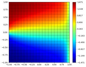
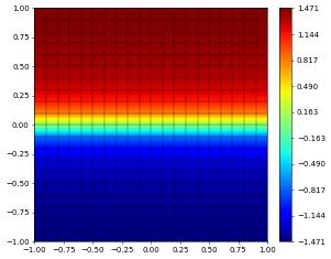
So far the example was not really advection dominated so we now repeat the experiment but set \(\varepsilon=1e-5\)

eps.value = 1e-5 # could also use scheme.model.eps = 1e-5
uh.interpolate(0)
scheme.solve(target=uh)

if parallel:
    gridView.writeVTK("u_h", pointdata=[uh])
else:
    uh.plot()

# for parallel runs skip 1d part
if parallel:
    sys.exit(0)

A linear transport problem

We now use a DG space to approximate the solution to the transport problem

\[\partial_t u + b\cdot \nabla u = f\]

with a constant transport velocity vector \(b\). We will solve the problem in one space dimension taking \(b=\frac{1}{2}\).

We first setup the 1D grid and the Discontinuous Galerkin space.

# remove later, shows same error: from dune.fem.space import dgonb as dgSpace
N = 200
gridView = leafGridView([0], [1], [N], overlap=1)
space    = dgSpace(gridView, order=1)

The space discretization uses the same upwind flux discussed already for the Advection-Diffusion problem in a previous example. This can be written as an ODE

\[\int_\Omega \partial_t u(t)\varphi_i = F_i(u(t))\]

where \((\varphi_i)_i\) is a basis of a DG space, i.e., \(\varphi_i=\varphi^E_l\) only has support on one element \(E\) of the grid. This leads to the matrix vector problem

\[M\frac{d}{dt} \vec{u}(t) = \vec{F}(\vec{u}(t))\]

where \(M\) is the mass matrix which in the case of a DG space is block diagonal - in fact with the dune.fem.space.dglegendre space the mass matrix is even diagonal. The ODE is thus of the form

\[\frac{d}{dt} \vec{u}(t) = M^{-1}\vec{F}(\vec{u}(t))\]

We discretize this ODE using an explicit two-step Runge-Kutta method with a fixed time-step \(\tau\). Given \(\vec{u}^n\) we define the solution at the next time step by

\[\vec{u}^{n+1} := \frac{1}{2}\Big(\vec{u}_1^{n+1} + \vec{u}_2^{n+1} \Big)\]

with \begin{align*} \vec{u}_1^{n+1} &= \vec{u}^n + \tau M^{-1}\vec{F}(\vec{u}^n) \\ \vec{u}_2^{n+1} &= \vec{u}_1^n + \tau M^{-1}\vec{F}(\vec{u}_1^n) \end{align*} This is Heun’s method.

We first setup the form for the right hand side \(\vec{F}\) which is very similar to the stationary case described above:

u    = TrialFunction(space)
v    = TestFunction(space)
n    = FacetNormal(space)
x    = SpatialCoordinate(space)

# transport direction and upwind flux
speed = 0.5
b     = as_vector([speed])
hatb  = (dot(b, n) + abs(dot(b, n)))/2.0
# boundary values (for left boundary)
dD    = conditional(x[0]<0.01,1,0)
g     = 1

# forms
advInternal = dot(-b*u, grad(v)) * dx
advSkeleton = jump(hatb*u)*jump(v) * dS
advBnd      = ( hatb*u + (dot(b,n)-hatb)*g )*v * dD*ds
form        = (advInternal + advSkeleton + advBnd)

We could use the standard approach based on the dune.fem.operator.galerkin construction but this requires adding the inverse mass operator later on. dune-fem provide an alternative approach where the operator automatically includes the inverse mass matrix:

from dune.fem.operator import molGalerkin as molOperator
op = molOperator(form)

So op(uh,res) applies the given operator to uh, applies the inverse mass matrix and stores the result in res. Consequently in our case, op(uh,res) computes \(M^{-1}\vec{F}(\vec{u}^n)\) as required.

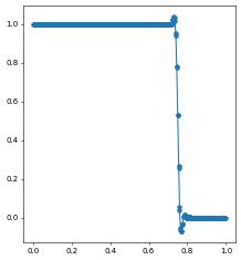
The remaining code is a rather standard time loop where we compute for a given old time step vector \(\vec{u}\) the new vector

\[\frac{1}{2}\Big( \vec{u}_1^{n+1} + \vec{u}_2^{n+1} \Big)\]

by applying the above operator twice.

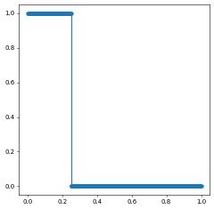
We show the transport of a a simple discontinuety:

uh = space.interpolate(conditional(x[0]<0.25,1,0), name="solution")
uh.plot()
w = uh.copy()
un = uh.copy()
cfl = 0.1
tau = cfl/(speed*N)

t = 0
while t<1:
    un.assign(uh)

    op(uh, w)
    uh.axpy(-tau,w)   # with numpy backend equivalent to 'uh.as_numpy[:] -= tau*w.as_numpy[:]'
    op(uh, w)
    uh.axpy(-tau,w)   # with numpy backend equivalent to 'uh.as_numpy[:] -= tau*w.as_numpy[:]'

    # with numpy backend the following is equivalent to
    # 'uh.as_numpy[:] = 0.5*(uh.as_numpy[:] + un.as_numpy[:])'
    uh *= 0.5
    uh.axpy(0.5,un)
    t += tau
uh.plot()

Todo

add some remarks on spectral dg

The dune.femdg module provides further methods for solving time dependent advection-diffusion problem. The module includes implicit-explicit Runge-Kutta methods and stabilization approaches for non-linear advection dominated models. This module is described in more details in other places in this tutorial.

This page was generated from the notebook discontinuousgalerkin_nb.ipynb and is part of the tutorial for the dune-fem python bindings