Overview

To facilitate rapid prototyping, the Dune Python bindings provide Python classes for all the core interfaces of Dune. This makes it easy to develop algorithms directly in Python which go beyond what is available through the Dune-Fem discretization module. This is especially of interest for pre- and postprocessing part of the overall simulation package. While most interface methods from the Dune-Fem package are high level, i.e., computationally expensive, many of the core Dune interface methods are not, i.e., the methods for computing the geometric representation of an element or the methods required to iterate over a grid. Consequently, depending on the requirements of the developed code parts, using the Dune core interfaces through Python could incur a too high hit on the performance of the code. Since the exported Python interfaces are very close to the original Dune C++ interfaces, transferring a Python prototype of the algorithm to C++ is mostly straightforward. A just in time compilation utility available in Dune-Python makes it then very easy to use these C++ algorithms from within Python.

In the following we briefly introduce the most important parts of the Dune core interface

Dense Vectors and the Geometry Classes

We start with a quick survey of Dune-Common and Dune-Geometry modules. The core module Dune-Common provides some classes for dense linear algebra.

import time, numpy, sys
import matplotlib.pyplot as pyplot
import dune.fem

from dune.common import FieldVector
x = FieldVector([0.25,0.25,0.25])
print(x)
print(numpy.array(x))

(0.250000, 0.250000, 0.250000)
[0.25 0.25 0.25]

The FieldVector and FieldMatrix classes are heavily used in the grid geometry realizations. The conceptional basis for these geometries is provided by Dune-Geometry, providing, for example, reference elements and quadrature rules.

import dune.geometry
geometryType = dune.geometry.simplex(2)
referenceElement = dune.geometry.referenceElement(geometryType)
print("\t".join(str(c) for c in referenceElement.corners))

for p in dune.geometry.quadratureRule(geometryType, 3):
    print("position:",p.position,f"({type(p.position)})", "weight:",p.weight,f"({type(p.weight)})")

(0.000000, 0.000000)    (1.000000, 0.000000)    (0.000000, 1.000000)
position: (0.333333, 0.333333) (<class 'dune.common.FieldVector_double_2'>) weight: -0.28125 (<class 'float'>)
position: (0.600000, 0.200000) (<class 'dune.common.FieldVector_double_2'>) weight: 0.2604166666666667 (<class 'float'>)
position: (0.200000, 0.600000) (<class 'dune.common.FieldVector_double_2'>) weight: 0.2604166666666667 (<class 'float'>)
position: (0.200000, 0.200000) (<class 'dune.common.FieldVector_double_2'>) weight: 0.2604166666666667 (<class 'float'>)

We can also obtain all weights and points stored in numpy arrays which can be useful to vectorize the computation of quadratures:

points,weights = dune.geometry.quadratureRule(geometryType, 3).get()
print("quadrature points:",points,f"({type(points)},{points.shape})")
print("quadrature weights:",weights,f"({type(weights)},{weights.shape})")

quadrature points: [[0.33333333 0.6        0.2        0.2       ]
 [0.33333333 0.2        0.6        0.2       ]] (<class 'numpy.ndarray'>,(2, 4))
quadrature weights: [-0.28125     0.26041667  0.26041667  0.26041667] (<class 'numpy.ndarray'>,(4,))

Grid Construction and Basic Interface

We now move on to the Dune-Grid module. First let us discuss different possibilities of constructing a grid.

Structured grids

We start with a structured grid. We saw in previous section the use of dune.grid.structuredGrid which is just a shortcut for setting up a Cartesian grid based on the yaspGrid grid manager which is part of dune.grid.

from dune.grid import cartesianDomain, yaspGrid
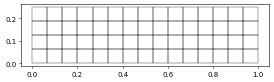
domain = cartesianDomain([0, 0], [1, 0.25], [15, 4])
yaspView = yaspGrid(domain)

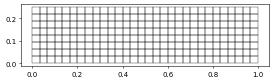
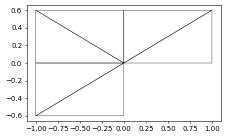
Let’s visualize the grid and then globally refine it once

yaspView.plot()
yaspView.hierarchicalGrid.globalRefine()
yaspView.plot()

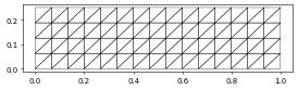
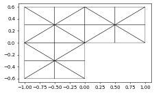
The dune.alugrid module provides 2d and 3d unstructured grids (both triangle and cubes). We can construct a triangle grid, visualize, and refine it in exactly the same way as the structured grid used above. We use dune.alugrid.aluConformGrid which uses newest vertex bisection to refine the grid. So one step of refinement only reduces the grid width by a factor of \(\sqrt2\). We we need two steps to half the grid width:

from dune.alugrid import aluConformGrid
aluView = aluConformGrid(domain)
aluView.plot()
aluView.hierarchicalGrid.globalRefine()
aluView.plot()
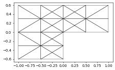
aluView.hierarchicalGrid.globalRefine()
aluView.plot()

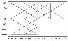
We can also provide the number of levels to refine to the globalRefine method:

domain = cartesianDomain([0, 0], [1, 0.25], [8, 2])
yaspView = yaspGrid(domain)
aluView = aluConformGrid(domain)

yaspView.hierarchicalGrid.globalRefine(2)
yaspView.plot()
aluView.hierarchicalGrid.globalRefine(4)
aluView.plot()

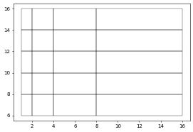
The dune.grid.yaspGrid grid manager also provides the option to construct tensor product grid. For a 2d grid one needs to provide a vector of x-coordinates \(x=(x_i)\) and y-coordinates \(y=(y_j)\) resulting in a grid with points \((x_i,y_j)\):

from dune.grid import tensorProductCoordinates
cst = dune.grid.tensorProductCoordinates([[1,2,4,8,16],[6,8,10,12,14,16]])
yaspView = dune.grid.yaspGrid(cst)
yaspView.plot()

Unstructured grids

General unstructured grids can be constructed by providing a dictionary containing vertex coordinate and element connectivity

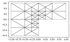
vertices = [(0,0), (1,0), (1,0.6), (0,0.6), (-1,0.6), (-1,0), (-1,-0.6), (0,-0.6)]
triangles = [(2,0,1), (0,2,3), (4,0,3), (0,4,5), (6,0,5), (0,6,7)]
aluView = aluConformGrid({"vertices": vertices, "simplices": triangles})
aluView.plot(figsize=(5,5))
aluView.hierarchicalGrid.globalRefine(2)
aluView.plot(figsize=(5,5))

An unstructured grid can also be constructed from a file. Currently gmsh and DGF are supported.

Local grid adaptivity

In addition to global refinement we can also pre process the grid by marking a subset of elements for local refinement.

from dune.grid import Marker
aluView.plot(figsize=(5,5))
for i in range(1,4):
    def mark(e):
        x = e.geometry.center
        return Marker.refine if x.two_norm < 0.64**i else Marker.keep
    aluView.hierarchicalGrid.adapt(mark)
    aluView.plot(figsize=(5,5))

from dune.alugrid import aluSimplexGrid
vertices = aluView.coordinates()
triangles = [aluView.indexSet.subIndices(e, 2) for e in aluView.elements]
aluView = aluSimplexGrid({"vertices": vertices, "simplices": triangles})

Tip

If discrete functions based on the dune.fem spaces have been constructed before local or global grid refinement is performed, the degree of freedom (dof) vectors will be resized but the data will be lost. Use dune.fem.adapt and dune.fem.globalRefine if data is supposed to be retained during grid modification. This is described in detail in the section on dynamic grid modification.

Basic information and iterators

We next discuss how to retrieve basic information from a constructed grid and iterate over its entities (i.e., elements, faces, edges, vertices, etc.).

vertices = [(0,0), (1,0), (1,1), (0,1)]
triangles = [(2,0,1), (0,2,3)]
unitSquare = aluSimplexGrid({"vertices": vertices, "simplices": triangles})
print(unitSquare.size(0),"elements and",unitSquare.size(2),"vertices")

for codim in range(0, unitSquare.dimension+1):
    for entity in unitSquare.entities(codim):
        print(", ".join(str(c) for c in entity.geometry.corners))

for edge in unitSquare.edges:
    print(", ".join(str(c) for c in edge.geometry.corners))

2 elements and 4 vertices
(1.000000, 1.000000), (1.000000, 0.000000), (0.000000, 0.000000)
(0.000000, 0.000000), (0.000000, 1.000000), (1.000000, 1.000000)
(0.000000, 0.000000), (1.000000, 0.000000)
(0.000000, 0.000000), (1.000000, 1.000000)
(0.000000, 0.000000), (0.000000, 1.000000)
(1.000000, 0.000000), (1.000000, 1.000000)
(1.000000, 1.000000), (0.000000, 1.000000)
(0.000000, 0.000000)
(1.000000, 0.000000)
(1.000000, 1.000000)
(0.000000, 1.000000)
(0.000000, 0.000000), (1.000000, 0.000000)
(0.000000, 0.000000), (1.000000, 1.000000)
(0.000000, 0.000000), (0.000000, 1.000000)
(1.000000, 0.000000), (1.000000, 1.000000)
(1.000000, 1.000000), (0.000000, 1.000000)

In the above we have used the geometry method on the entity which provides the geometric mapping between the reference element of the entity and it’s position in physical space. We have used the corners method to retrieve corners of the entity. Other properties and methods are available to provide volume or the integration element needed to compute quadratures of a grid function over the element - which is discussed in the next section.

Using grid functions

This is a fundamental concept in any grid based discretization package. These are functions that can be evaluated given an entity in the grid and a local coordinate within the reference element of that entity.

Tip

in the following we will use the gridFunction decorator provided by dune.fem. A very similar decorator is also available in dune.grid but the latter does not provide the option to use the grid functions in ufl expressions.

@dune.fem.function.gridFunction(aluView, name="cos", order=3)
def f(x):
    return numpy.cos(2.*numpy.pi/(0.3+abs(x[0]*x[1])))

@dune.fem.function.gridFunction(aluView, name="hat0", order=3)
def hat0(element,hatx):
    return 1-hatx[0]-hatx[1]

hatx = FieldVector([1./3., 1./3.])
maxValue = max(f(e, hatx) for e in f.gridView.elements)

maxValue = max(f(e.geometry.toGlobal(hatx)) for e in f.gridView.elements)

hat0.plot()
f.plot()
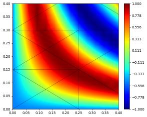
f.plot(level=3,xlim=[0,0.4], ylim=[0,0.4])

We can now use the quadrature rules discuss at the beginning of this chapter to compute the integral over each element of the grid function.

from dune.geometry import quadratureRules
rules = quadratureRules(5)
integral = 0
for e in aluView.elements:
    geo = e.geometry
    for qp in rules(e.type):
        x,w = qp.position, qp.weight
        integral += f(e,x)*w*geo.integrationElement(x)
print("integral of function 'f':",integral)

integral of function 'f': 0.07942992585030194

There are some approach available to improve the efficiency of the computation of integrals since this is an important component of many grid based schemes. Especially, using vectorization can greatly reduce the complexity of the above loop:

integral = 0
for e in aluView.elements:
    # obtain numpy arrays containing the points and weights and then call
    # required functions using these vectors with requiring a loop
    points, weights = rules(e.type).get()
    ies = e.geometry.integrationElement(points)
    values = f(e,points)
    integral += numpy.sum(values*ies*weights,axis=-1)
print("integral of function 'f':",integral)

integral of function 'f': 0.07942992585030188

Now a vector valued function

# an easy case
dimR = 2
@dune.fem.function.gridFunction(aluView, name="g", order=3)
def g(x):
    return [numpy.cos(2.*numpy.pi/(0.3+abs(x[0]*x[1])))]*dimR
# bit more complex to code
@dune.fem.function.gridFunction(aluView, name="g", order=3)
def g(x):
    if type(x[0]) is float:
        return [numpy.cos(2.*numpy.pi/(0.3+abs(x[0]*x[1]))),1]
    else:
        return [numpy.cos(2.*numpy.pi/(0.3+abs(x[0]*x[1]))),[1]*len(x[0])]
integral = g.dimRange*[0]
for e in aluView.elements:
    # obtain numpy arrays containing the points and weights and then call
    # required functions using these vectors with requiring a loop
    points, weights = rules(e.type).get()
    ies = e.geometry.integrationElement(points)
    values = g(e,points)
    integral += numpy.sum(values*ies*weights,axis=-1)
print("integral of function 'g':",integral)

integral of function 'g': [0.07942993 1.8       ]

Importing user defined C++ code

To achieve close to native efficiency the Python prototype can be easily reimplemented as a C++ function and the algorithm module used for just in time compilation. This is discussed in a later section based on some examples.

Attaching Data to the Grid

To attach data to the entities in a grid, each Dune grid has an IndexSet which provides a consecutive, zero starting integer for the set of entities of a given geometry type, i.e., entities sharing the same reference element, like all triangles or all cubes. This can be used to attach data to these entities stored in random access containers like numpy arrays. To simplify the process further a mapper can be used which is initialized with the data layout, i.e., the number of degrees of freedom that is supposed to be attached to every entity with a given geometry type.

In the following we first construct a mapper for a 2d cube grid attaching 2 dofs to each element (codimension 0), 4 to each edge (codimension 1), and 3 to each vertex (codimension 2):

layout = [2,4,3]
mapper = unitSquare.mapper([2, 4, 3])
print( mapper.size, sum([layout[c]*unitSquare.size(c) for c in range(3)]) )

36 36

We can also use the reference element types from dune.geometry to define the layout

layout = {dune.geometry.quadrilateral: 4, dune.geometry.triangle: 1}
mapper = unitSquare.mapper(layout)

Finally here is an example of using the mapper to attach one degree of freedom per vertex and using that to define a piecewise linear Lagrange interpolation:

def interpolate(grid):
    mapper = grid.mapper({dune.geometry.vertex: 1})
    data = numpy.zeros(mapper.size)
    for v in grid.vertices:
        data[mapper.index(v)] = f(v.geometry.center)
    return mapper, data

mapper, data = interpolate(aluView)
@dune.fem.function.gridFunction(aluView, name="p12d", order=1)
def p12dEvaluate(e, x):
    bary = 1-x[0]-x[1], x[0], x[1]
    idx = mapper.subIndices(e, 2)
    return sum(b * data[i] for b, i in zip(bary, idx))

We can use a grid function to compute the error of the Lagrange interpolation at the barycenter of each triangle:

@dune.fem.function.gridFunction(aluView, name="error", order=3)
def error(e, x):
    return abs(p12dEvaluate(e, x)-f(e, x))
hatx = FieldVector([1./3., 1./3.])
print(max(error(e, hatx) for e in aluView.elements))

1.6026566867981322

Tip

the mapper describe here provides a slightly extended interface compared to the mappers available from discrete spaces in dune.fem. While the mappers from the grid provide methods like subIndices and similar the mapper from the space only provide a method to obtain all indices attached to a given (codimension 0) entity. This method is also available in the mappers from the grid.

for i,e in enumerate(aluView.elements):
    print(mapper(e))
    if i==4: break

[0 1 2]
[0 3 1]
[3 4 1]
[5 4 3]
[2 6 0]

Output of Grid and Visualization of Data

We already used matplotlib to plot the grid and grid functions. For more flexible plotting Dune relies on vtk and it easy to write suitable files.

Matplotlib

We have seen many examples already of using matplotlib to show the grid and grid functions. The most straightforward way is to use the plot method. We first show three plots using matplotlib

Tip

the plot method will only work on 1d or 2d grids.

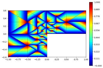
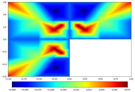
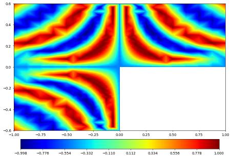
p12dEvaluate.plot(figsize=(9,9), gridLines=None, colorbar="horizontal")
f.plot(level=2, figsize=(9,9), gridLines=None, colorbar="horizontal")
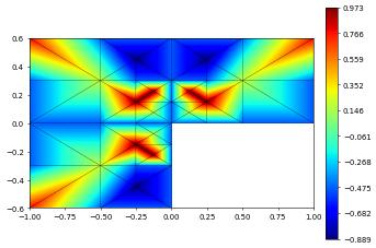
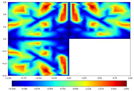
error.plot(level=2, figsize=(9,9), gridLines=None, colorbar="horizontal")

Paraview (vtu/vtk files)

Now we write out vtu files and use pvpython to prduce similar but 3d plots of the same functions

pd = {"exact": f, "discrete": p12dEvaluate, "error": error}
aluView.writeVTK("interpolation", pointdata=pd)

aluView.writeVTK("interpolation_subsampled", subsampling=2, pointdata=pd)

Here are pngs generated with paraview from the above output: The discrete interpolation 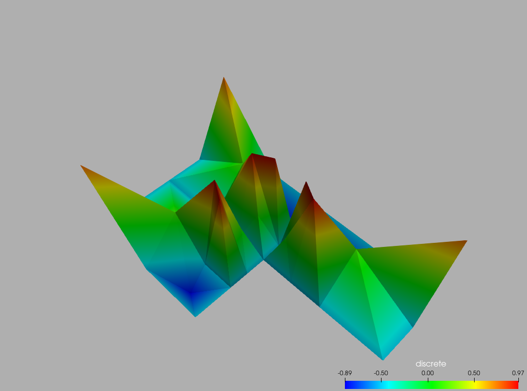A zoom in 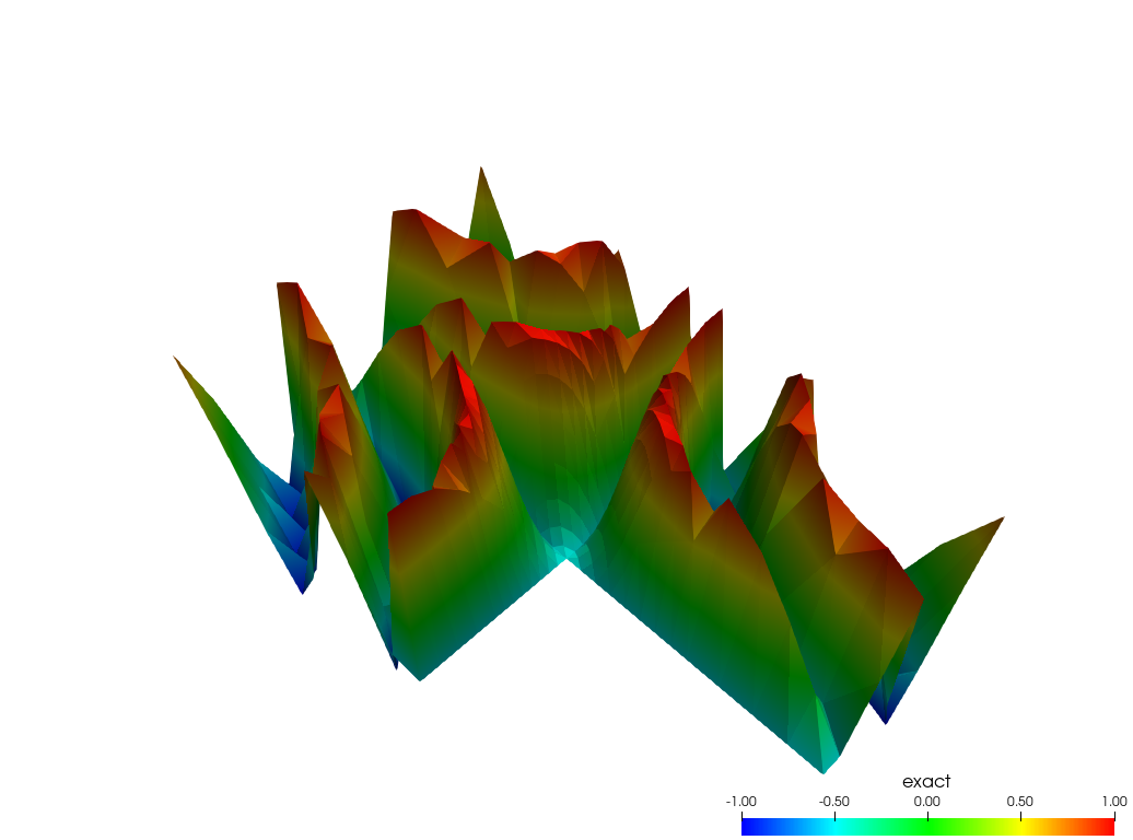The interpolation error on the subsampled grid

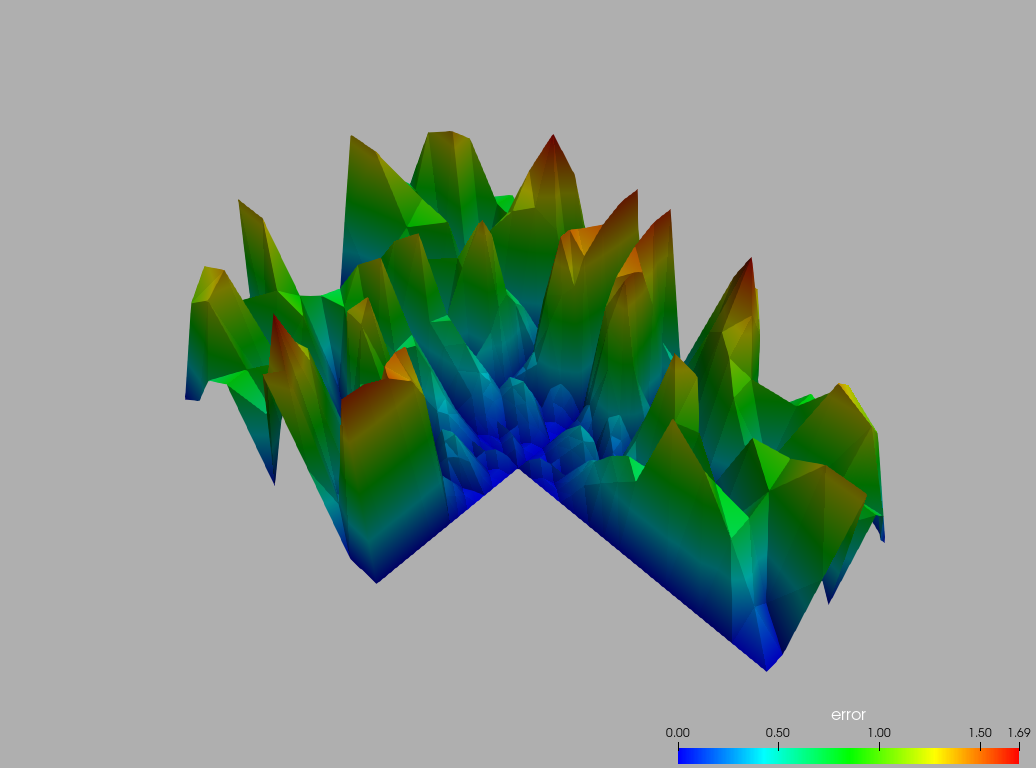
Mayavi

Mayavi can also be used to plot grid function in Python. This approach relies on methods to extract numpy representations of the grid data structure and values of a given grid function.

level = 3
triangulation = f.gridView.triangulation(level)
z = f.pointData(level)[:,0]
try:
    from mayavi import mlab
    from mayavi.tools.notebook import display
    mlab.init_notebook("png")
    mlab.figure(bgcolor = (1,1,1))
    s = mlab.triangular_mesh(triangulation.x, triangulation.y, z*0.5,
                             triangulation.triangles)
    display( s )
    # mlab.savefig("mayavi.png", size=(400,300))
    mlab.close(all=True)
except ImportError:
    print("mayavi module not found so not rendering plot - ignored")
    pass

mayavi module not found so not rendering plot - ignored

Low level output

Todo

add some information on the tessellate and related methods, e.g., coordinates , polygons , tessellate , triangulation

gridView.triangulation(level=0, *, partition=...)  (for 2d grids)
     Returns: matplotlib.tri.Triangulation structure

More general methods

coordinates(...)
   Returns: `numpy` array with the coordinates of all vertices in the grid in
            the format `[ [x_1,y_1], [x_2,y_2], ..., [x_N,y_N] ]` for example
            in 2d (will be filled up by zeros if dimworld is larger
            than the world dimension of the view.
polygons(...)   Store the grid in numpy arrays.
   Returns: coordinate array storing the vertex coordinate of each polygon
            in the grid.
tessellate(level=0,dimworld=gv.dimensionworld) or tessellate(level=0,*,partition,dimworld=gv.dimensionworld)
  Generated a possibly refined tessellation using only simplices.
     Args: level: virtual refinement level to use to generate the tessellation
     Returns: (coordinates,simplices) where coordinates is a `numpy` array
              of the vertex coordinates (padded by to `dimworld` is needed)
              (e.g. in 2d `[ [x_1,y_1,0], [x_2,y_2,0], ..., [x_N,y_N],0 ]`
              if `dimworld` is set to 3 - default is no padding,
              `dimworld` less than actual world dimension of grid is ignored)
              and simplices is a `numpy` array of the vertices of the simplices
              (e.g. in 2d `[s_11,s_12,s_13], [s_21,s_22,s_23], ..., [s_N1,s_N2,s_N3] ]` )

Partner methods on grid function:

gridFunction.cellData, gridFunction.pointData, gridFunction.polygonData

Todo

add something on intersections

This page was generated from the notebook dune-corepy_nb.ipynb and is part of the tutorial for the dune-fem python bindings