Note
This document is part of the dune-fem tutorialJupyter notebook (_nb.ipynb) or as Python script (.py)More General Boundary Conditions
So far we have used Dirichlet and trivial Neumann boundary conditions. Here we discuss how to impose other conditions like general Neumann, Robin and more general Dirichlet conditions. We will show how to add these to the model and how to prescribe different conditions for different components of the solution in the case of vector valued PDEs.
Dirichlet boundary conditions
To fix Dirichlet boundary conditions \(u=g\) on part of the boundary \(\Gamma\subset\partial\Omega\) the central class is dune.ufl.DirichletBC which takes three arguments: the discrete function space for \(u\), the function \(g\) given by a UFL expression, and a description of \(\Gamma\). There are different ways to do this. If the final argument is omitted or None the condition is applied to the whole domain, a integer \(s>0\) can be provided which can be set to
describe a part of the boundary during grid construction as described at the end of this section. Finally a UFL condition can be used, i.e., x[0]<0.
For vector valued functions \(u\) the value function \(g\) can be a UFL vector or a list. In the later case a component of None can be used to describe components which are not to be constrained by the boundary condition.
[1]:
from matplotlib import ticker
from matplotlib import pyplot as plt
from dune.fem.plotting import plotComponents
import numpy, io
from dune.grid import structuredGrid as leafGridView
from dune.fem.space import lagrange as solutionSpace
from dune.fem.scheme import galerkin as solutionScheme
from dune.fem.function import gridFunction
from dune.ufl import DirichletBC, Constant
from ufl import TestFunction, TrialFunction, SpatialCoordinate,\
dx, ds, grad, inner, sin, pi
gridView = leafGridView([0, 0], [1, 1], [4, 4])
vecSpace = solutionSpace(gridView, dimRange=2, order=2)
x = SpatialCoordinate(vecSpace)
vec = vecSpace.interpolate([0,0], name='u_h')
uVec,vVec = TrialFunction(vecSpace), TestFunction(vecSpace)
a = inner(grad(uVec), grad(vVec)) * dx
a += ( ( 10*(1-2*uVec[1])+uVec[0] ) * vVec[0] +\
( 10*sin(2*pi*x[1]) + (1-2*uVec[0])**2*uVec[1] ) * vVec[1]
) * dx
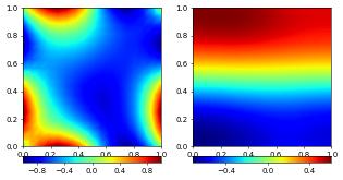
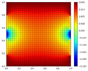
# Define Dirichlet boundary conditions for first component on all boundaries
bc = DirichletBC(vecSpace,[sin(2*pi*(x[0]+x[1])),None])
vecScheme = solutionScheme( [a == 0, bc],
parameters={"linear.tolerance": 1e-9} )
vecScheme.solve(target=vec)
plotComponents(vec, gridLines=None, level=2,
colorbar={"orientation":"horizontal", "ticks":ticker.MaxNLocator(nbins=4)})
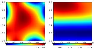
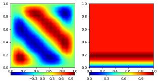
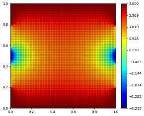
To prescribe \(u_2=1\) at the bottom boundary is easily achieve by providing multiple instances of the dune.ufl.DiricheltBC class:
[2]:
bcBottom = DirichletBC(vecSpace,[sin(2*pi*(x[0]+x[1])),1],x[1]<1e-10)
vecScheme = solutionScheme( [a == 0, bc, bcBottom],
        parameters={"linear.tolerance": 1e-9} )
vecScheme.solve(target=vec)
plotComponents(vec, gridLines=None, level=2,
               colorbar={"orientation":"horizontal", "ticks":ticker.MaxNLocator(nbins=4)})

We can also use general grid functions (including discrete functions) for the boundary conditions in the same way we could use grid functions anywhere within the UFL forms. We could for example fix the boundary values of the first component using the discrete solution from the previous computation by writing bc = DirichletBC(vecSpace,[vec[0],None]) Since this would just be an approximation to the actual boundary condition the overall results would not be identical to the previous version. We
therefore do not use the discrete solution to describe the boundary conditions but instead use other forms of grid functions. The following two code snippets lead to the same results as above:
[3]:
test = vec.copy()
test.clear()
@gridFunction(gridView ,name="bnd",order=2)
def bnd(x):
    return [numpy.sin(2*numpy.pi*(x[0]+x[1])),1]
bcBottom = DirichletBC(vecSpace,bnd,x[1]<1e-10)
vecScheme = solutionScheme( [a == 0, bc, bcBottom],
        parameters={"linear.tolerance": 1e-9} )
vecScheme.solve(target=test)
plotComponents(test, gridLines=None, level=2,
               colorbar={"orientation":"horizontal", "ticks":ticker.MaxNLocator(nbins=4)})
assert sum([ abs(td-vd) for td,vd in zip(test.dofVector, vec.dofVector)] ) /\
       len(vec.dofVector) < 1e-8
As with other grid functions we can also use C++ code snippets. to define the Dirichlet conditions.
Accessing the Dirichlet degrees of freedom
We provide a few methods to apply or otherwise access information about the Dirichlet constraints from an existing scheme.
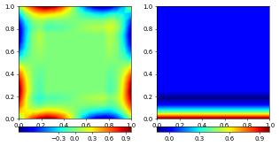
The following shows how to set all degrees of freedom on the Dirichlet boundary to zero. For a more realistic example see the second approach in the section on solving Dirichlet Eigenvalue problems.
[4]:
for i in vecScheme.dirichletIndices():
    vec.dofVector[i] = 0
Tip
The dirichletIndices method takes as optional argument an id which then returns the list of indices of degrees of freedom on the boundary with that id. See further down for a discussion on boundary ids.
We have set all degrees of freedom on the boundary to zero. In this example the Dirichlet boundary was specified by the two DirichletBC instances bc and bcBottom. The first specified that for the first component the whole boundary was Dirichlet while specifying nothing for the second component. The second then set Dirichlet conditions for the second component along the lower boundary. Consequently, the solution should now be zero along the whole boundary in the first component, and
zero along the lower boundary for the second:
[5]:
plotComponents(vec, gridLines=None, level=2,
               colorbar={"orientation":"horizontal", "ticks":ticker.MaxNLocator(nbins=4)})
It is sometimes necessary to set all degrees of freedom on the boundary to zero, to be equal to some other function, or to as an interpolation of the boundary data provided to the scheme. To this end the operators/schemes provide methods setConstraints. To cover the cases detailed above, there are three versions of this method:
the first takes a discrete function and sets the Dirichlet dofs to the boundary data provided in the
DirichletBCstructure.The second version takes a range vector and a discrete function; this version can used for example to set the values at the boundary to zero, e.g.,
op.setConstraints(0, uh)or for a vector functionop.setConstraints([0,]*space.dimension, vec_h).Finally there is a version taking a grid function and a discrete function
op.setConstraints(g, uh)which sets the dofs at the boundary so thatuh=gat the Dirichlet boundary.
We use the first version to set the data at the boundary first having cleared the discrete function. As second example we interpolate the bnd grid function and then set all boundary dofs to 0. Recall that the second component has no Dirichlet boundary conditions set at the lower boundary.
[6]:
vec.clear()
vecScheme.setConstraints(vec)
plotComponents(vec, gridLines=None, level=2,
               colorbar={"orientation":"horizontal", "ticks":ticker.MaxNLocator(nbins=4)})
vec.interpolate(bnd)
vecScheme.setConstraints([0,]*len(vec), vec)
plotComponents(vec, gridLines=None, level=2,
               colorbar={"orientation":"horizontal", "ticks":ticker.MaxNLocator(nbins=4)})
Neumann and Robin boundary conditions
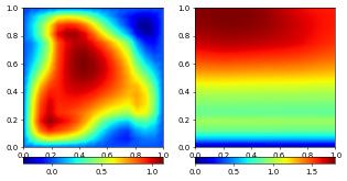
Neumann boundary flux are added to the ufl form by using the measure ufl.ds. By default they will be added to all boundaries for which no Dirichlet conditions have been prescribed. In the above example we prescribed no Dirichlet conditions to the second component at both vertical and the top boundary using the dune.ufl.DirichletBC instance bc. This leads to zero fluxes (natural boundary conditions) being used there. To add some (here nonlinear) Neumann boundary conditions for the
second component at these three sides we can simply add an additional term to a:
[7]:
a  = a + uVec[0]*uVec[0] * vVec[1] * ds
vecScheme = solutionScheme( [a == 0, bc],
        parameters={"linear.tolerance": 1e-9} )

vecScheme.solve(target=vec)

plotComponents(vec, gridLines=None, level=2,
               colorbar={"orientation":"horizontal", "ticks":ticker.MaxNLocator(nbins=4)})
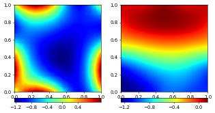
Robin boundary conditions can be handled in the same way using the ufl.ds measure.
Using boundary ids (and some more complex examples)
Up until now we have used UFL boolean expressions to define the subset of the boundary where a Dirichlet condition should be applied. In many cases different parts of the boundary are already marked with ids (integers) during grid construction. These ids can also be used to define where boundary conditions are to be applied. At the moment it is possible to use boundary ids using a dict to define the grid, using boundary tagging with gmsh, or constructing the grid using the Dune Grid
Format (dgf) reader. Please consult the documentation of the DGF file format for details. In the section on other examples given for grid construction provides more details.
Cartesian boundary ids
For Cartesian grids the boundary ids are rather fixed and pre-described due to implementation specifics. The numbering of the boundary edges follows the numbering of faces of the DUNE reference elements but starts from 1. For example, in 2d the boundary ids are left=1, right=2, bottom=3, top=4 and in 3d bottom=5, top=6. For grids implementing a true Cartesian grids, like YaspGrid,
this is fixed. Altering this numbering can only be done by using an unstructured grid, e.g. ALUGrid. See the grid construction section to get an idea how this is done.
Note
Boundary ids and refinement: Boundary ids only allow to tell apart intersections with the domain boundary on the macro level of a grid. Descendants of macro intersections on the domain boundary inherit the boundary id of their parent.
We can use the utility grid function dune.fem.function.boundaryFunction to visualize the boundary ids.
[8]:
from dune.fem.function import boundaryFunction
boundaryFunction(gridView).plot()
Mixing different types of boundary conditions
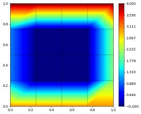
These ids can be used as third argument in the DirichletBC constructor and also in the boundary measure ufl.ds as shown in the following examples solving a Laplace problem with a combination of Neumann, Robin, and Dirichlet boundary conditions.
In this example the boundary conditions are
left and right boundary (id=1 and id=2): Robin boundary conditions \(\nabla u\cdot n + u = -10\) for \(y\in[0.4,0.6]\) and natural boundary conditions (\(\nabla u\cdot n=0\)) otherwise.
bottom boundary (id=3): Neumann conditions \(\nabla u\cdot n=2\)
top boundary (id=4): Dirichlet conditions \(u=1\) for \(x\in [0.3,0.6]\) and natural boundary conditions (\(\nabla u\cdot n=0\)) otherwise.
[9]:
from dune.ufl import BoundaryId
from ufl import ds, grad, dot, inner, conditional, eq, And, FacetNormal, Not

gridView.hierarchicalGrid.globalRefine(3)
space = solutionSpace(gridView, order=2)
x,n = SpatialCoordinate(space), FacetNormal(space)
u,v = TrialFunction(space), TestFunction(space)
a  = inner(grad(u), grad(v)) * dx

fbnd  = (u-10 * v *                    # middle of left and right boundary
         conditional(abs(x[1]-0.5)<0.1,1,0) ) * ds( (1,2) )
fbnd += 2 * v * ds(3)                  # bottom boundary
dbc   = DirichletBC(space, 1,          # middle of top boundary
           And( eq(BoundaryId(space),4), abs(x[0]-0.5)<0.2 ))

scheme   = solutionScheme( [a == fbnd, dbc] )
solution = space.interpolate(0, name='u_h')
scheme.solve(target=solution)
solution.plot()
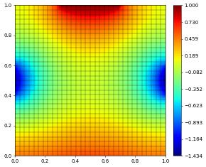
The next example has a slightly more complex setup at the boundary:
left and right (id=1 and id=2): for \(y\in[0.4,0.6]\) we set Neumann conditions \(\nabla u\cdot n=-50\)
left and right (id=1 and id=2): for \(y\in[0.2,0.8]\setminus [0.4,0.6]\) we set Dirichlet conditions \(u=1\)
rest of boundary: 3
[10]:
fbnd  = (-50 * v *                     # middle of left and right boundary
         conditional(abs(x[1]-0.5)<0.1,1,0) ) * ds( (1,2) )
dbc   = [ DirichletBC(space, 1,        # not middle of left and right boundary
            And( And( BoundaryId(space)<=2,
                 abs(x[1]-0.5)>0.1 ), abs(x[1]-0.5)<0.3 ) ),
          DirichletBC(space, 3,        # not middle of left and right boundary
            Not( And(BoundaryId(space)<=2,abs(x[1]-0.5)<0.3) ) ), ]
scheme   = solutionScheme( [a == fbnd, *dbc] )
solution = space.interpolate(0, name='u_h')
scheme.solve(target=solution)
solution.plot()
Let check if that solution makes sense…
[11]:
gridView.hierarchicalGrid.globalRefine(1)
scheme.solve(target=solution)
solution.plot()
Using a dictionary to define the grid with boundary ids
We have already used a dictionary to define the vertices and the elements (in this case cubes) of the grid. In addition we can use the boundaries key. In 2d the value for this key is a list of two vertex indices and if boundary ids are to be used three integers, where the first is the id and the other two are the vertex indices of the edge. Finally we can define a default value for the boundary id used for boundary segments not added otherwise - if this is not provided the default id
will be fixed to ‘1’:
Note
the following only works with the grid managers from the dune.alugrid package:
[12]:
import dune.alugrid
domain = {'vertices': [[0.        , 0.        ],
                       [1.        , 0.        ],
                       [1.        , 1.1       ],
                       [0.        , 1.1       ],
                       [0.25      , 0.        ],
                       [0.5       , 0.        ],
                       [0.75      , 0.        ],
                       [1.        , 0.19166667],
                       [1.        , 0.55      ],
                       [1.        , 0.74166667],
                       [0.75      , 1.1       ],
                       [0.5       , 1.1       ],
                       [0.25      , 1.1       ],
                       [0.        , 0.74166667],
                       [0.        , 0.55      ],
                       [0.        , 0.19166667],
                       [0.25      , 0.35833333],
                       [0.25      , 0.55      ],
                       [0.25      , 0.90833333],
                       [0.5       , 0.19166667],
                       [0.5       , 0.55      ],
                       [0.5       , 0.74166667],
                       [0.75      , 0.35833333],
                       [0.75      , 0.55      ],
                       [0.75      , 0.90833333]],
          'cubes': [[ 0,  4, 15, 16],
                    [15, 16, 14, 17],
                    [14, 17, 13, 18],
                    [13, 18,  3, 12],
                    [ 4,  5, 16, 19],
                    [16, 19, 17, 20],
                    [17, 20, 18, 21],
                    [18, 21, 12, 11],
                    [ 5,  6, 19, 22],
                    [19, 22, 20, 23],
                    [20, 23, 21, 24],
                    [21, 24, 11, 10],
                    [ 6,  1, 22,  7],
                    [22,  7, 23,  8],
                    [23,  8, 24,  9],
                    [24,  9, 10,  2]],
          'boundaries': [[2, 0, 4],
                         [2, 4, 5],
                         [2, 5, 6],
                         [2, 6, 1],
                         [2, 1, 7],
                         [2, 7, 8],
                         [2, 8, 9],
                         [2, 9, 2]],
          'defaultBndId': 5}
gridView = dune.alugrid.aluCubeGrid(domain)
gridView.plot()
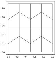
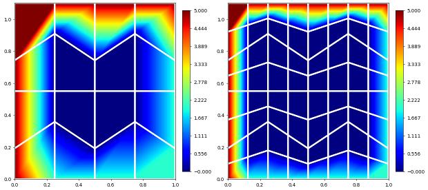
As already mentioned refining the grid does not change the boundary ids:
[13]:
fig, axs = plt.subplots(1, 2, figsize=(12,6))
boundaryFunction(gridView).plot(gridLines="white", linewidth=3, figure=(fig,axs[0]))
gridView.hierarchicalGrid.globalRefine(1)
boundaryFunction(gridView).plot(gridLines="white", linewidth=3, figure=(fig,axs[1]))
Note
This document is part of the dune-fem tutorialJupyter notebook (.ipynb) or as Python script (.py)