Problem Description
This example considers two-phase porous-media flow. In all that follows, we assume that the flow is immiscible and incompressible with no mass transfer between phases. A detailed description of the mathematical model and parameters can be found [DKKN18].
[1]:
try:
    import dune.femdg
except ImportError:
    print("This example needs 'dune.femdg' - skipping")
    import sys
    sys.exit(0)

from matplotlib import pyplot

import numpy
from ufl import *
from dune.ufl import Space, Constant

import dune.fem as fem
import dune.create as create
from dune.generator import algorithm
from dune.common import FieldVector
from dune.grid import cartesianDomain, Marker
from dune.fem.function import levelFunction, gridFunction
from dune.fem import integrate
from dune.plotting import plotPointData as plot

from limit import createOrderRedcution, createLimiter

fem.threading.use = 4
Some parameters
[2]:
maxLevel  = 3
maxOrder  = 3
dt        = 5.
endTime   = 800.
coupled   = False
tolerance = 3e-2
penalty   = 5 * (maxOrder * ( maxOrder + 1 ))
newtonParameters = {"tolerance": tolerance,
                    "verbose": "false", "linear.verbose": "false",
                    "linabstol": 1e-8, "reduction": 1e-8}
Defining the model
using a Brooks Corey pressure law
[3]:
def brooksCorey(P,s_n):
    s_w = 1-s_n
    s_we = (s_w-P.s_wr)/(1.-P.s_wr-P.s_nr)
    s_ne = (s_n-P.s_nr)/(1.-P.s_wr-P.s_nr)
    if P.useCutOff:
        cutOff = lambda a: min_value(max_value(a,0.00001),0.99999)
        s_we = cutOff(s_we)
        s_ne = cutOff(s_ne)
    kr_w = s_we**((2.+3.*P.theta)/P.theta)
    kr_n = s_ne**2*(1.-s_we**((2.+P.theta)/P.theta))
    p_c  = P.pd*s_we**(-1./P.theta)
    dp_c = P.pd * (-1./P.theta) * s_we**(-1./P.theta-1.) * (-1./(1.-P.s_wr-P.s_nr))
    l_n  = kr_n / P.mu_n
    l_w  = kr_w / P.mu_w
    return p_c,dp_c,l_n,l_w
Constants and domain description for anisotropic lens test
[4]:
class AnisotropicLens:
    dimWorld = 2
    domain   = cartesianDomain([0,0.39],[0.9,0.65],[15,4])
    x        = SpatialCoordinate(triangle)

    g     = [0,]*dimWorld ; g[dimWorld-1] = -9.810 # [m/s^2]
    g     = as_vector(g)
    r_w   = 1000.  # [Kg/m^3]
    mu_w  = 1.e-3  # [Kg/m s]
    r_n   = 1460.  # [Kg/m^3]
    mu_n  = 9.e-4  # [Kg/m s]

    lens = lambda x,a,b: (a-b)*                (conditional(abs(x[1]-0.49)<0.03,1.,0.)*                 conditional(abs(x[0]-0.45)<0.11,1.,0.))                + b

    p_c = brooksCorey

    Kdiag = lens(x, 6.64*1e-14, 1e-10) # [m^2]
    Koff  = lens(x, 0,-5e-11)          # [m^2]
    K     = as_matrix( [[Kdiag,Koff],[Koff,Kdiag]] )

    Phi   = lens(x, 0.39, 0.40)             # [-]
    s_wr  = lens(x, 0.10, 0.12)             # [-]
    s_nr  = lens(x, 0.00, 0.00)             # [-]
    theta = lens(x, 2.00, 2.70)             # [-]
    pd    = lens(x, 5000., 755.)            # [Pa]

    #### initial conditions
    p_w0 = (0.65-x[1])*9810.       # hydrostatic pressure
    s_n0 = 0                       # fully saturated
    # boundary conditions
    inflow = conditional(abs(x[0]-0.45)<0.06,1.,0.)*             conditional(abs(x[1]-0.65)<1e-8,1.,0.)
    J_n  = -5.137*1e-5
    J_w  = 1e-20
    dirichlet = conditional(abs(x[0])<1e-8,1.,0.) +                conditional(abs(x[0]-0.9)<1e-8,1.,0.)
    p_wD = p_w0
    s_nD = s_n0

    q_n  = 0
    q_w  = 0

    useCutOff = False

P = AnisotropicLens()
Setup grid, discrete spaces and functions
[5]:
grid = create.view("adaptive", "ALUCube", P.domain, dimgrid=2)

if coupled:
    spc          = create.space("dglegendrehp", grid, dimRange=2, order=maxOrder)
else:
    spc1         = create.space("dglegendrehp", grid, dimRange=1, order=maxOrder)
    spc          = create.space("product", spc1,spc1, components=["p","s"] )

solution     = spc.interpolate([0,0], name="solution")
solution_old = spc.interpolate([0,0], name="solution_old")
sol_pm1      = spc.interpolate([0,0], name="sol_pm1")
intermediate = spc.interpolate([0,0], name="iterate")
persistentDF = [solution,solution_old,intermediate]

fvspc        = create.space("finitevolume", grid, dimRange=1, storage="numpy")
estimate     = fvspc.interpolate([0], name="estimate")
estimate_pm1 = fvspc.interpolate([0], name="estimate-pm1")
[6]:
uflSpace = Space((P.dimWorld,P.dimWorld),2)
u        = TrialFunction(uflSpace)
v        = TestFunction(uflSpace)
cell     = uflSpace.cell()
x        = SpatialCoordinate(cell)
tau      = Constant(dt, name="timeStep")
beta     = Constant(penalty, name="penalty")

p_w  = u[0]
s_n  = u[1]

p_c,dp_c,l_n,l_w = P.p_c(s_n=intermediate[1])
Bulk terms
[7]:
dBulk_p  = P.K*( (l_n+l_w)*grad(p_w) + l_n*dp_c*grad(s_n) )
dBulk_p += -P.K*( (P.r_n*l_n+P.r_w*l_w)*P.g )
bulk_p   = -(P.q_w+P.q_n)
dBulk_s  = P.K*l_n*dp_c*grad(s_n)
dBulk_s += P.K*l_n*(grad(p_w)-P.r_n*P.g)
bulk_s   = -P.q_n
Boundary and initial conditions
[8]:
p_D, s_D = P.p_wD, P.s_nD,
p_N, s_N = P.J_w+P.J_n, P.J_n
p_0, s_0 = P.p_w0, P.s_n0
Bulk integrals
[9]:
form_p = ( inner(dBulk_p,grad(v[0])) + bulk_p*v[0] ) * dx
form_s = ( inner(dBulk_s,grad(v[1])) + bulk_s*v[1] ) * dx
Boundary fluxes
[10]:
form_p += p_N * v[0] * P.inflow * ds
form_s += s_N * v[1] * P.inflow * ds
DG terms
[11]:
def sMax(a): return max_value(a('+'), a('-'))
n         = FacetNormal(cell)
hT        = MaxCellEdgeLength(cell)
he        = avg( CellVolume(cell) ) / FacetArea(cell)
heBnd     = CellVolume(cell) / FacetArea(cell)
k         = dot(P.K*n,n)
lambdaMax = k('+')*k('-')/avg(k)
def wavg(z): return (k('-')*z('+')+k('+')*z('-'))/(k('+')+k('-'))
Penalty terms (including dirichlet boundary treatment)
[12]:
p_c0,dp_c0,l_n0,l_w0 = P.p_c(0.5)
penalty_p = [beta*lambdaMax*sMax(l_n0+l_w0),
             beta*k*(l_n0+l_w0)]
penalty_s = [beta*lambdaMax*sMax(l_n0*dp_c0),
             beta*k*(l_n0*dp_c0)]
form_p += penalty_p[0]/he * jump(u[0])*jump(v[0]) * dS
form_s += penalty_s[0]/he * jump(u[1])*jump(v[1]) * dS
form_p += penalty_p[1]/heBnd * (u[0]-p_D) * v[0] * P.dirichlet * ds
form_s += penalty_s[1]/heBnd * (u[1]-s_D) * v[1] * P.dirichlet * ds
Consistency terms
[13]:
form_p -= inner(wavg(dBulk_p),n('+')) * jump(v[0]) * dS
form_s -= inner(wavg(dBulk_s),n('+')) * jump(v[1]) * dS
form_p -= inner(dBulk_p,n) * v[0] * P.dirichlet * ds
form_s -= inner(dBulk_s,n) * v[1] * P.dirichlet * ds
Time discretization
[14]:
form_s = P.Phi*(u[1]-solution_old[1])*v[1] * dx + tau*form_s
Stabilization (Limiter)
[15]:
limiter = createLimiter( spc, limiter="scaling" )
tmp = solution.copy()
def limit(target):
    tmp.assign(target)
    limiter(tmp,target)
Time stepping Converting UFL forms to scheme
[16]:
if coupled:
    form = form_s + form_p
    tpModel = create.model( "integrands", grid, form == 0)
    # tpModel.penalty  = penalty
    # tpModel.timeStep = dt
    scheme = create.scheme("galerkin", tpModel, spc, ("suitesparse","umfpack"),
                     parameters={"newton." + k: v for k, v in newtonParameters.items()})
else:
    uflSpace1 = Space((P.dimWorld,P.dimWorld),1)
    u1        = TrialFunction(uflSpace1)
    v1        = TestFunction(uflSpace1)
    form_p = replace(form_p, { u:as_vector([u1[0],intermediate.s[0]]),
                             v:as_vector([v1[0],0.]) } )
    form_s = replace(form_s, { u:as_vector([solution[0],u1[0]]),
                             intermediate:as_vector([solution[0],intermediate[1]]),
                             v:as_vector([0.,v1[0]]) } )
    form = [form_p,form_s]
    tpModel = [create.model( "integrands", grid, form[0] == 0),
               create.model( "integrands", grid, form[1] == 0)]
    # tpModel[0].penalty  = penalty
    # tpModel[1].penalty  = penalty
    # tpModel[1].timeStep = dt
    scheme = [create.scheme("galerkin", m, s, ("suitesparse","umfpack"),
                     parameters={"newton." + k: v for k, v in newtonParameters.items()})
                for m,s in zip(tpModel,spc.components)]
Stopping condition for iterative approaches
[17]:
def errorMeasure(w,dw):
    rel = integrate([w[1]**2,dw[1]**2], order=5, gridView=grid)
    return numpy.sqrt(rel[1]) < tolerance * numpy.sqrt(rel[0])
Iterative schemes (iterative or impes-iterative)
[18]:
def step():
    n = 0
    solution_old.assign(solution)
    while True:
        intermediate.assign(solution)
        if coupled:
            scheme.solve(target=solution)
        else:
            scheme[0].solve(target=solution.p)
            scheme[1].solve(target=solution.s)
        limit(solution)
        n += 1
        # print("step",n,flush=True)
        if errorMeasure(solution,solution-intermediate) or n==20:
            break
HP Adpativity
Setting up residual indicator
[19]:
uflSpace0 = Space((P.dimWorld,P.dimWorld),1)
v0        = TestFunction(uflSpace0)

Rvol = P.Phi*(u[1]-solution_old[1])/tau - div(dBulk_s) - bulk_s
estimator = hT**2 * Rvol**2 * v0[0] * dx +      he * inner(jump(dBulk_s), n('+'))**2 * avg(v0[0]) * dS +      heBnd * (s_N + inner(dBulk_s,n))**2 * v0[0] * P.inflow * ds +      penalty_s[0]**2/he * jump(u[1])**2 * avg(v0[0]) * dS +      penalty_s[1]**2/heBnd * (s_D - u[1])**2 * v0[0] * P.dirichlet * ds
estimator = replace(estimator, {intermediate:u})

estimatorModel = create.model("integrands", grid, estimator == 0)
# estimatorModel.timeStep = dt
# estimatorModel.penalty  = penalty
estimator = create.operator("galerkin", estimatorModel, spc, fvspc)
Marker for grid adaptivity (h)
[20]:
hTol = 1e-16                           # changed later
def markh(element):
    center = element.geometry.referenceElement.center
    eta    = estimate.localFunction(element).evaluate(center)[0]
    if eta > hTol and element.level < maxLevel:
      return Marker.refine
    elif eta < 0.01*hTol:
      return Marker.coarsen
    else:
      return Marker.keep
Marker for space adaptivity (p)
[21]:
pTol = 1e-16
def markp(element):
    center = element.geometry.referenceElement.center
    r      = estimate.localFunction(element).evaluate(center)[0]
    r_p1   = estimate_pm1.localFunction(element).evaluate(center)[0]
    eta = abs(r-r_p1)
    polorder = spc.localOrder(element)
    if eta < pTol:
        return polorder-1 if polorder > 1 else polorder
    elif eta > 100.*pTol:
        return polorder+1 if polorder < maxOrder else polorder
    else:
        return polorder
Operator for projecting into space with a reduced order on every element
[22]:
orderreduce = createOrderRedcution( spc )
Main program
Pre adapt the grid
[23]:
hgrid = grid.hierarchicalGrid
hgrid.globalRefine(1)
for i in range(maxLevel):
    print("pre adaptive (",i,"): ",grid.size(0),end="\n")
    solution.interpolate( as_vector([p_0,s_0]) )
    limit(solution)
    step()
    estimator(solution, estimate)
    hgrid.mark(markh)
    fem.adapt(persistentDF)

print("final pre adaptive (",i,"): ",dt,grid.size(0),end="\n")
pre adaptive ( 0 ):  240
pre adaptive ( 1 ):  231
pre adaptive ( 2 ):  363
final pre adaptive ( 2 ):  5.0 273
Define the constant for the h adaptivity
[24]:
solution.interpolate( as_vector([p_0,s_0]) )
limit(solution)
estimator(solution, estimate)
timeTol = sum(estimate.dofVector) / endTime
print('Using timeTol = ',timeTol, end='\n')
Using timeTol = 3.216131221875019e-15
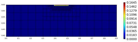
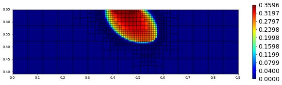
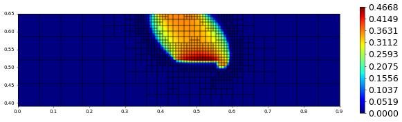
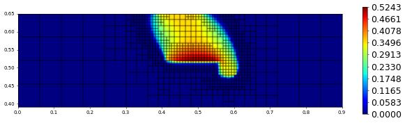
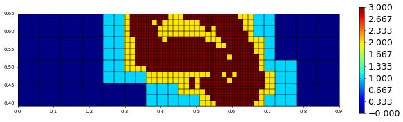
Time loop
[25]:
t = 0
saveStep = 0
while t < endTime:
step()
# h adaptivity
hTol = timeTol * dt / grid.size(0)
estimator(solution, estimate)
hgrid.mark(markh)
fem.adapt(persistentDF)
# p adaptivity
estimator(solution, estimate)
orderreduce(solution,sol_pm1)
estimator(sol_pm1, estimate_pm1)
fem.spaceAdapt(spc, markp, persistentDF)
t += dt
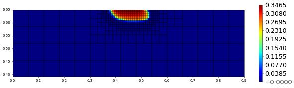
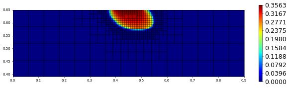
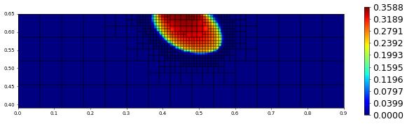
if t>=saveStep:
print(t,grid.size(0),sum(estimate.dofVector),hTol,"# timestep",flush=True)
plot(solution[1],figsize=(15,4))
saveStep += 100
5.0 240 0.0 5.890350223214321e-17 # timestep
100.0 363 0.0 4.46684891927086e-17 # timestep
200.0 498 0.0 3.248617395833353e-17 # timestep
300.0 582 0.0 2.748830104166683e-17 # timestep
400.0 669 0.0 2.4145129293356e-17 # timestep
500.0 774 0.0 2.0856882113326973e-17 # timestep
600.0 885 0.0 1.8232036405187182e-17 # timestep
700.0 1017 0.0 1.585863521634625e-17 # timestep
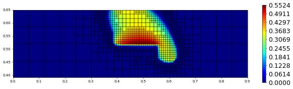
800.0 1134 0.0 1.4255900806183596e-17 # timestep

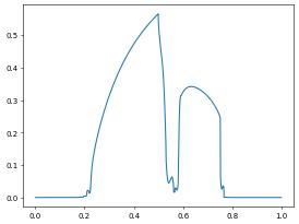
Postprocessing Show solution along a given line
[26]:
x0 = FieldVector([0.25,  0.65])
x1 = FieldVector([0.775, 0.39])
p,v = algorithm.run('sample', 'utility.hh', solution, x0, x1, 1000)

x = numpy.zeros(len(p))
y = numpy.zeros(len(p))
l = (x1-x0).two_norm
for i in range(len(x)):
    x[i] = (p[i]-x0).two_norm / l
    y[i] = v[i][1]
pyplot.plot(x,y)
[26]:
[<matplotlib.lines.Line2D at 0x7f8d9dbbceb0>]
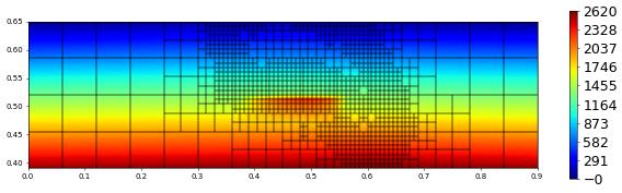
[27]:
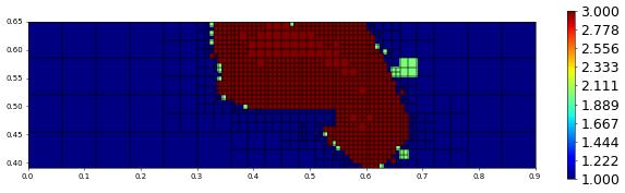
from dune.fem.function import levelFunction
@gridFunction(gridView=grid,name="polOrder",order=0)
def polOrder(e,x):
return [spc.localOrder(e)]
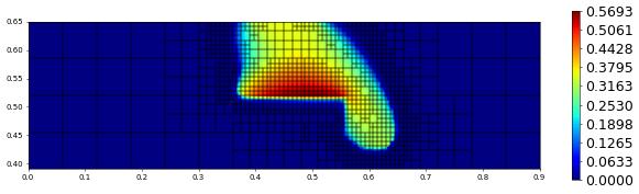
plot(solution[0],figsize=(15,4))
plot(solution[1],figsize=(15,4))
plot(polOrder,figsize=(15,4))
plot(levelFunction(grid),figsize=(15,4))
This page was generated from
the notebook twophaseflow_nb.ipynb
and is part of the tutorial for the dune-fem python bindings
![]()