Note
This document is part of the dune-fem tutorialJupyter notebook (_nb.ipynb) or as Python script (.py)Cahn-Hilliard
In this script we show how to use the \(C^1\) non-conforming virtual element space to solve the Cahn-Hilliard equation. We use a fully implicit scheme here. You can find more details in [DH21]
[1]:
try:
    import dune.vem
except:
    print("This example needs 'dune.vem' - skipping")
    import sys
    sys.exit(0)
from matplotlib import pyplot
import random
from dune.grid import cartesianDomain, gridFunction
import dune.fem
from dune.fem.plotting import plotPointData as plot
from dune.fem.function import discreteFunction

from ufl import *
import dune.ufl

dune.fem.threading.use = 4
Grid and space construction - we use a cube grid here:
[2]:
order        = 3
polyGrid = dune.vem.polyGrid( cartesianDomain([0,0],[1,1],[30,30]), cubes=True)
testSpaces = [ [0], [order-3,order-2], [order-4] ]
# testSpaces   = [ [0,0],[order-4,order-3], [order-4] ]
space = dune.vem.vemSpace(polyGrid, order=order, testSpaces=testSpaces)
To define the mathematical model, let \(\psi\colon{\mathbb R} \rightarrow \mathbb{R}\) be defined as \(\psi(x) = \frac{(1-x^2)^2}{4}\) and let \(\phi(x) = \psi(x)^{\prime}\). The strong form for the solution \(u\colon \Omega \times [0,T] \rightarrow {\mathbb R}\) is given by \begin{align*} \partial_t u - \Delta (\phi(u)-\epsilon^2 \Delta u) = 0 \quad &\text{in} \ \Omega \times [0,T] ,\\ u(\cdot,0) = u_0(\cdot) \quad &\text{in} \ \Omega,\\ \partial_n u = \partial_n \big( \phi(u) - \epsilon^2\Delta u \big) = 0 \quad &\text{on} \ \partial \Omega \times [0,T]. \end{align*}
We use a backward Euler discretization in time and will fix the constant further down:
[3]:
t     = dune.ufl.Constant(0,"time")
tau   = dune.ufl.Constant(0,"dt")
eps   = dune.ufl.Constant(0,"eps")
df_n  = discreteFunction(space, name="oldSolution") # previous solution
x     = SpatialCoordinate(space)
u     = TrialFunction(space)
v     = TestFunction(space)

H     = lambda v: grad(grad(v))
laplace = lambda v: H(v)[0,0]+H(v)[1,1]
a     = lambda u,v: inner(H(u),H(v))
b     = lambda u,v: inner( grad(u),grad(v) )
W     = lambda v: 1/4*(v**2-1)**2
dW    = lambda v: (v**2-1)*v

equation = ( u*v + tau*eps*eps*a(u,v) + tau*b(dW(u),v) ) * dx == df_n*v * dx

dbc = [dune.ufl.DirichletBC(space, 0, i+1) for i in range(4)]

# energy
Eint  = lambda v: eps*eps/2*inner(grad(v),grad(v))+W(v)
Next we construct the scheme providing some suitable expressions to stabilize the method
[4]:
biLaplaceCoeff = eps*eps*tau
diffCoeff      = 2*tau
massCoeff      = 1
scheme = dune.vem.vemScheme(
                       [equation, *dbc],
                       solver=("suitesparse","umfpack"),
                       hessStabilization=biLaplaceCoeff,
                       gradStabilization=diffCoeff,
                       massStabilization=massCoeff,
                       boundary="derivative") # only fix the normal derivative = 0
To avoid problems with over- and undershoots we project the initial conditions into a linear lagrange space before interpolating into the VEM space:
[5]:
def initial(x):
    h = 0.01
    g0 = lambda x,x0,T: conditional(x-x0<-T/2,0,conditional(x-x0>T/2,0,sin(2*pi/T*(x-x0))**3))
    G  = lambda x,y,x0,y0,T: g0(x,x0,T)*g0(y,y0,T)
    return 0.5*G(x[0],x[1],0.5,0.5,50*h)
initial = dune.fem.space.lagrange(polyGrid,order=1).interpolate(initial(x),name="initial")
df = space.interpolate(initial, name="solution")
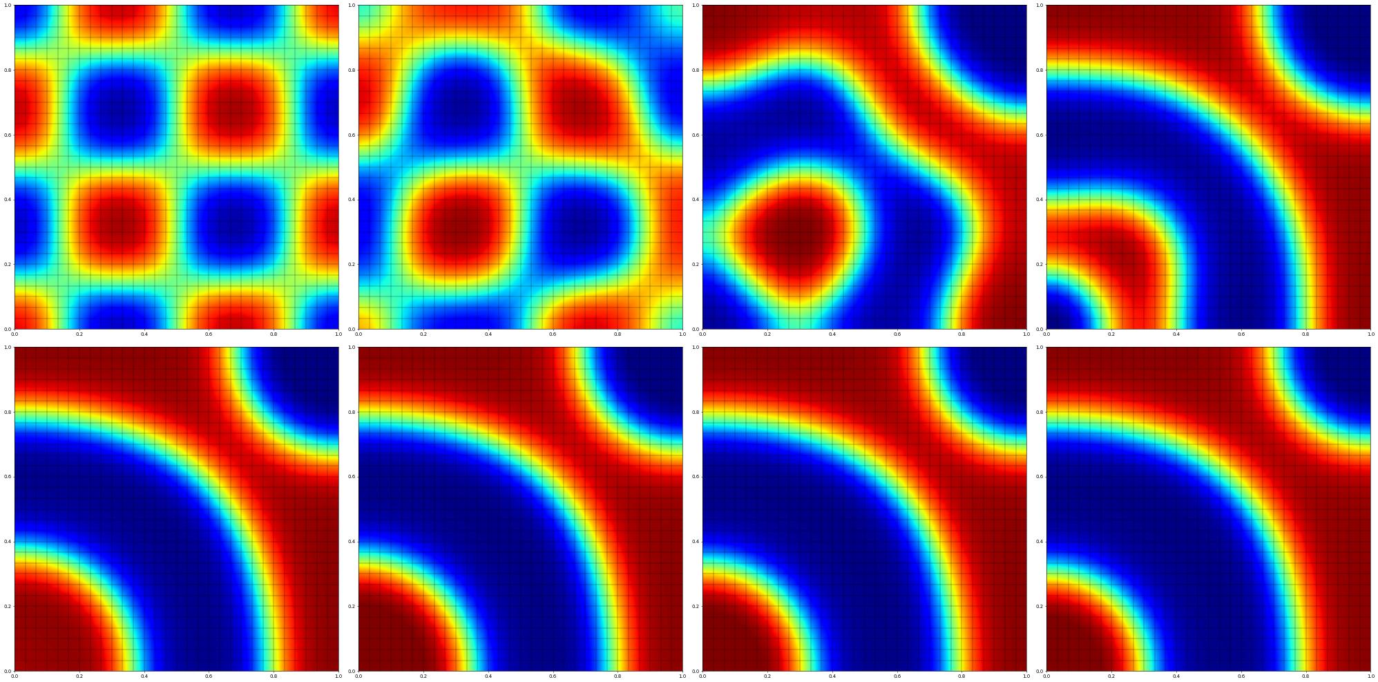
Finally the time loop - for the final coarsening phase (time greater than 0.8) we increase the time step a bit:
[6]:
t.value = 0
eps.value = 0.05

fig = pyplot.figure(figsize=(30,30))
count = 0
pos = 1
while t.value < 2.15:
    if t.value < 0.6:
        tau.value = 1e-02
    else:
        tau.value = 5e-02
    df_n.assign(df)
    info = scheme.solve(target=df)
    t.value += tau
    count += 1
    if count % 10 == 0:
        df.plot(figure=(fig,330+pos),colorbar=None,clim=[-1,1])
        energy = dune.fem.integrate(Eint(df),order=3)
        print("[",pos,"]",t.value,tau.value,energy,info,flush=True)
        pos += 1
[ 1 ] 0.09999999999999999 0.01 0.2110245353293364 {'converged': True, 'iterations': 2, 'linear_iterations': 2, 'timing': [0.650024995, 0.418875944, 0.231149051]}
[ 2 ] 0.20000000000000004 0.01 0.19940917553129997 {'converged': True, 'iterations': 3, 'linear_iterations': 3, 'timing': [0.906761835, 0.584721513, 0.322040322]}
[ 3 ] 0.3000000000000001 0.01 0.15197040274240364 {'converged': True, 'iterations': 3, 'linear_iterations': 3, 'timing': [0.887617047, 0.5690280320000001, 0.3185890149999999]}
[ 4 ] 0.4000000000000002 0.01 0.13249947517006797 {'converged': True, 'iterations': 3, 'linear_iterations': 3, 'timing': [0.950122445, 0.638276069, 0.311846376]}
[ 5 ] 0.5000000000000002 0.01 0.11180986038847346 {'converged': True, 'iterations': 3, 'linear_iterations': 3, 'timing': [0.893942199, 0.591658868, 0.30228333100000004]}
[ 6 ] 0.6000000000000003 0.01 0.10910600941981931 {'converged': True, 'iterations': 2, 'linear_iterations': 2, 'timing': [0.582064538, 0.371933117, 0.21013142100000004]}
[ 7 ] 1.1000000000000008 0.05 0.09508742037332195 {'converged': True, 'iterations': 3, 'linear_iterations': 3, 'timing': [0.916158624, 0.589836713, 0.3263219110000001]}
[ 8 ] 1.6000000000000012 0.05 0.06999066566664237 {'converged': True, 'iterations': 3, 'linear_iterations': 3, 'timing': [0.926699411, 0.5977880339999999, 0.32891137700000006]}
[ 9 ] 2.100000000000001 0.05 0.05876099820814534 {'converged': True, 'iterations': 2, 'linear_iterations': 2, 'timing': [0.617005029, 0.38524934099999997, 0.23175568800000002]}
Note
This document is part of the dune-fem tutorialJupyter notebook (.ipynb) or as Python script (.py)