Stokes-Darcy equation

Table of Contents

• Introduction
• Mathematical background
• Setup and initialization
• Define problem data
• Create grid
• Setup subdomains and boundary patches
• Create finite element basis
• Create matrix, vector, and constraints data structures
• Assemble the variational problem
• Solve the algebraic problem
• Write solution to VTK
• Error handling

Full code of this example This example on gitlab

Introduction

The following example shows how to solve a Stokes-Darcy problem for coupled free and ground water flow. The problem couples the Stokes and Darcy equation in two non-overlapping subdomains. At the subdomain interface it imposes a Beavers-Joseph-Saffman condition for the tangential velocity of the Stokes flow and a Neumann-Neumann coupling for the normal velocity of Stokes and Darcy flow. In particular the example demonstrates how to

• define and setup subdomains,
• restrict finite element spaces to subdomains,
• assemble problems on subdomains,
• assemble coupling terms at subdomain interfaces.

Mathematical background

Consider a domain \(\Omega \subset \mathbb{R}^d\) decomposed according to \( \overline{\Omega} = \overline{\Omega_S} \cup \overline{\Omega_D}\) into two non-overlapping subdomains \(\Omega_S\) and \(\Omega_D\). We assume the Dirichlet boundary condition \(u=u_D\) for the Stokes problem on \( \Gamma_{S} \subset \partial \Omega_S \cap \partial \Omega\) and \(\phi=\phi_D\) for the Darcy problem on \( \Gamma_{D} \subset \partial \Omega_D \cap \partial \Omega\). Then the weak forms of the Stokes and Darcy problem in \(\Omega_S\) and \(\Omega_D\), respectively, are given by:

Find \( u \in H^1_{\Gamma_{S},u_D}(\Omega_S)^d, p \in L^2(\Omega)\) such that

\[ \begin{align*} \int_{\Omega_S} 2\nu \varepsilon(u) \colon \varepsilon(v) \,dx - \int_{\Omega_S} \operatorname{div}(v) p \,dx&= 0 &&\forall v\in H^1_{\Gamma_{S},0}(\Omega_S)^d,\\ - \int_{\Omega_S} \operatorname{div}(u) q \,dx&= 0 &&\forall q\in L^2(\Omega_S). \end{align*} \]

Find \( \varphi \in H^1_{\Gamma_{D},\varphi_D}(\Omega_D)\) such that

\[ \begin{align*} \int_{\Omega_D} K \nabla \varphi \cdot \nabla \psi \,dx &= 0 &&\forall \psi\in H^1_{\Gamma_{D},0}(\Omega_D). \end{align*} \]

Here we used the symmetric gradient \( \varepsilon(v) = \frac{1}{2}(\nabla v + \nabla v^T)\), the viscosity \( \nu>0\), the permeability \( K>0\), and the spaces \(H^1_{\Gamma_S,w}(\Omega_S)^d = \{v \in H^1(\Omega_S)^d\,|\, v|_{\Gamma_S} = w\}\) and \(H^1_{\Gamma_D,w}(\Omega_D) = \{v \in H^1(\Omega_D)\,|\, v|_{\Gamma_D} = w\}\).

On the subdomain boundary \( \Gamma = \overline{\Omega_S} \cap \overline{\Omega_D}\) the equations are coupled by a Neumann-Neumann coupling of the normal components. Furthermore the Beavers-Joseph-Saffman condition is imposed for the tangential Stokes flux of the Stokes velocity on \(\Gamma\). This leads to the following weak form of the coupled problem.

Find \((u,p,\varphi) \in V_{u_d,\varphi_D}\) such that:

\[ \begin{align*} A((u,p,\varphi), (v,q,\psi)) &= 0 && \forall (v,q,\psi) \in V_{0,0} \end{align*} \]

on the product spaces \(V_{v,\psi} = H^1_{\Gamma_S,v}(\Omega_S)^d \times L^2(\Omega_S) \times H^1_{\Gamma_D,\psi}(\Omega_D)\). The bilinear form \(A : V_{u_d,\varphi_D} \times V_{0,0} \to \mathbb{R}\) is given by

\[ \begin{multline*} A((u,p,\varphi), (v,q,\psi)) = \underbrace{a_S(u,v) + b(u,q) + b(v,p)}_{\text{Stokes}} + \underbrace{a_D(\varphi,\psi)}_{\text{Darcy}}\\ + \underbrace{a_{BJS}(u,v)}_{\text{Beavers–Joseph–Saffman}} + \underbrace{c((u,\varphi), (v,\psi))}_{\text{coupling}} \end{multline*} \]

with the contributions

\[ \begin{align*} a_S(u,v) &= \int_{\Omega_S} 2\nu \varepsilon(u) \colon \varepsilon(v) \,dx &&\text{(Stokes diffusion)},\\ b(v,q) &= -\int_{\Omega_S} \operatorname{div}(v)q \,dx &&\text{(Stokes incompressibility)},\\ a_D(\varphi,\psi) &= \int_{\Omega_D} K \nabla \varphi \cdot \nabla \psi \,dx, &&\text{(Darcy diffusion)},\\ a_{BJS}(u,v) &= \int_\Gamma \alpha (P_\tau u) \cdot v \,ds &&\text{(Beavers–Joseph–Saffman)},\\ c((u,\varphi), (v,\psi)) &= \int_\Gamma (g \varphi v - \psi u) \cdot n \,ds &&\text{(Neumann–Neumann coupling)}. \end{align*} \]

Here \(n:\Gamma \to \mathbb{R}^d\) is the unit normal vector to \(\Gamma\) which by convention points from \(\Omega_S\) to \(\Omega_D\), \(P_{\tau}:\Gamma \to \mathbb{R}^{d \times d}\) is the orthogonal projection on the tangent space of \(\Gamma\), \(g \in \mathbb{R} \geq 0\) is the gravitational acceleration constant, and \(\alpha = \alpha_{BJS} K^{-\frac{1}{2}}\) where \(\alpha_{BJS} >0 \) is a constant for the Beavers-Joseph-Saffman condition.

The problem is discretized using Taylor-Hood mixed finite elements for the Stokes fluid and classical Lagrange elements for the Darcy pressure using order \(k+1\) for the Stokes velocity, order \(k\) for the Stokes pressure, and order \(k+1\) for the Darcy pressure.

Setup and initialization

After including the required headers the main() function first creates a simple logger that allows to write log messages to std::cout. The logger will prefix log messages with the time passed since the program was started and since the last log message using the given format string. Afterward MPI is initialized, passing the command line arguments.

int main (int argc, char *argv[]) try
{
 
  auto log = Dune::Fufem::makeLogger(std::cout, "[% 8.3f] [% 8.3f] ");
 
  Dune::MPIHelper::instance(argc, argv);
 
  log("MPI initialized");

Define problem data

Next we define some problem data. Simple parameters can be set using command line arguments. To this end we make use of Dune::ParameterTree which is a tree-of-strings data structure. Here parameters.get<T>("key", defaultValue) reads the value with the respective key from the ParameterTree and converts it to the type T if it exists, otherwise the defaultValue is used. By parsing the command line into the ParameterTree we can pass parameters using command line arguments of the form -viscosity 1.0.

  auto parameters = Dune::ParameterTree();
  Dune::ParameterTreeParser::readOptions(argc, argv, parameters);
 
  auto nu           = parameters.get<double>("viscosity", 1.0);
  auto K            = parameters.get<double>("permeability", 1.0e-2);
  auto alpha_BJS    = parameters.get<double>("alpha_BJS", 1.0);
  auto g            = parameters.get<double>("gravity", 1.0);
  auto meshFile     = parameters.get<std::string>("meshFile", "stokes-darcy.msh");
  auto StokesID     = parameters.get<int>("StokesID", 1);
  auto DarcyID      = parameters.get<int>("DarcyID", 2);
  auto refinements  = parameters.get<std::size_t>("refinements", 2);
 
  log("Command line processed");

The Dirichlet values for the Stokes velocity and Darcy pressure are defined using lambda expressions.

  constexpr std::size_t dim = 2;
 
  auto stokesVelocityDirichletValues = [](auto x)
  {
    return Dune::FieldVector<double,dim>{1.0, 0.0};
  };
 
  auto darcyDirichletValues = [](auto x)
  {
    return 0;
  };

Create grid

The grid is created using a so called GridFactory. The latter is filled using the Dune::GmshReader which allows to read a mesh file generated by the Gmsh program.

  using Grid = Dune::UGGrid<dim>;
 
  auto factory = Dune::GridFactory<Grid>();
  auto reader = Dune::GmshReader<Grid>(meshFile, factory);
  auto gridPtr = factory.createGrid();
  auto& grid = *gridPtr;

Note

For the given example we provide both, the geometry description stokes-darcy.geo and the mesh file stokes-darcy.msh. The former has been generated from the latter using the command

gmsh stokes-darcy.geo -1 -2 -o stokes-darcy.msh

The Gmsh file format allows to attach data (in the form of int values) to elements and boundary intersections. Instead of using the raw interface of the GmshReader to extract this data, we here use the convenience classes ElementData and BoundaryData. These classes store the respective data in a persistent form that also allows to be used after grid refinement. Both can either be used like a random access container, using the index of an element or the boundary-segment-index of an intersection, or as a callback that directly maps element or intersection to the data.

  auto elementData = Dune::Fufem::ElementData(reader, factory, grid);
  auto boundaryData = Dune::Fufem::BoundaryData(reader, factory, grid);

Note

Since there are no element indices with respect to the whole grid, the ElementData class strictly speaking depends on the a so called GridView instead of the grid. By only providing the grid, it implicitly uses the leaf GridView as default, which is almost always the one of interest. However, we could alternatively provide a GridView directly here.

Next we refine the grid globally as many times as requested with the -refinements option. All further computations will be done on the leaf GridView of the grid which consists of the most refined elements. Since refining the grid changes element indices, we need to announce this to the ElementData container using its update(gridView) method. Afterwards we can request the data associated to the elements and boundary intersections of the respective grid view.

  grid.globalRefine(refinements);
 
  auto gridView = grid.leafGridView();
 
  elementData.update(gridView);
 
  log("Grid refined");

Setup subdomains and boundary patches

The subdomains are represented by SubDomain objects from the dune-functions module. Since the feature is quite new, it is for now contained in the namespace Dune::Functions::Experimental. The creation of a subdomains is simple. We first create a SubDomain object on the gridView. Then we loop over all elements of the grid and insert the elements into the SubDomain identified by the elementData read from the mesh file.

  using Dune::Functions::Experimental::SubDomain;
  using Dune::Functions::Experimental::SubDomainInterface;
 
  auto stokesDomain = SubDomain(gridView);
  for(auto&& element : elements(gridView))
    if (elementData(element) == StokesID)
      stokesDomain.insertElement(element);
 
  log(Dune::formatString("Stokes domain contains %d elements", stokesDomain.indexSet().size(0)));
 
  auto darcyDomain = SubDomain(gridView);
  for(auto&& element : elements(gridView))
    if (elementData(element) == DarcyID)
      darcyDomain.insertElement(element);
 
  log(Dune::formatString("Darcy domain contains %d elements", darcyDomain.indexSet().size(0)));

Since we later want to assemble coupling terms at the subdomain interface \(\Gamma = \overline{\Omega_S}\cap\overline{\Omega_D}\) we also create a SubDomainInterface object for the two subdomains. This represents the set of all intersections of grid elements from the two subdomains. The order of the two subdomains passed as arguments does matter, since the intersections will always be oriented from the first to the second subdomain.

Note

The dune grid interface allows to traverse all intersections of a grid element with its adjacent elements. Consequently the two adjacent elements of such an intersection are called inside and outside and the normal vector of an intersection is oriented from inside to outside. When visiting the same geometrical intersection from the two adjacent elements the respective intersection objects behave similar, but the role of inside and outside and thus the normal vector is flipped.

Here we orient the SubDomainInterface from Stokes- to Darcy-subdomain such that the normal vectors of the interface are outward normals of the Stokes-subdomain.

  auto interface = SubDomainInterface(stokesDomain, darcyDomain);
 
  log("Interface created");

Similar to the SubDomain class the BoundaryPatch handle a subset of the grid. In contrast to the former, the latter represents a subset of the boundary intersections. Here we use two boundary patches for the Dirichlet boundary of the Stokes and Darcy domain and insert the intersections according to their associated Id. To traverse the boundary we use the Dune::Fufem::Boundary class which encapsulates all boundary intersections as an iterable range.

  auto stokesDirichletBoundary = Dune::Fufem::BoundaryPatch(gridView);
  for (const auto& intersection : Dune::Fufem::Boundary(gridView))
    if (boundaryData(intersection) == StokesID)
      stokesDirichletBoundary.insertFace(intersection);
 
  auto darcyDirichletBoundary = Dune::Fufem::BoundaryPatch(gridView);
  for (const auto& intersection : Dune::Fufem::Boundary(gridView))
    if (boundaryData(intersection) == DarcyID)
      darcyDirichletBoundary.insertFace(intersection);
 
  log("Dirichlet boundaries created");

Create finite element basis

The basis of a finite element space is created by passing a descriptor of the basis and a GridView to the makeBasis(...) function. The product space of different bases can be created using composite(basis1, basis2, basis3, ...) while the k-fold product of the same basis can be created using power<k>(basis). Nesting these expressions allows to construct bases or arbitrarily nested product spaces.

Note

The additional arguments to composite and power control how the basis functions will be indexed. Using flatLexicographic leads to flat indices from \(\mathbb{N}_0\). Passing other flags one can also create multi-indices which allows to address nested containers.

For the particular problem we use a Taylor-Hood basis with the orders 2 and 1 for velocity and pressure for the Stokes problem and a Lagrange basis of order 2 for the Darcy problem. Since the bases for the Stokes and Darcy problem should only have support in the respective subdomains, we restrict the bases to the corresponding SubDomain objects. I.e. the basis functions obtained using restrict(lagrange<k>(), darcyDomain) will only have support in the Darcy-subdomain and will look like the Lagrange-basis for a grid only covering this domain.

All the described utilities for creating bases are provided by the dune-functions module in the namespace Dune::Functions::BasisFactory, with the exception of the recently added restrict(...) function which is contained in Dune::Functions::Experimental::BasisFactory.

  using namespace Dune::Functions::BasisFactory;
  using namespace Dune::Functions::Experimental::BasisFactory;
 
  constexpr std::size_t maxOrder = 2;
  auto basis = makeBasis(gridView,
      composite(
        restrict(
          composite(
            power<dim>(lagrange<maxOrder>(), flatInterleaved()),
            lagrange<maxOrder-1>(),
            flatLexicographic()
          ), stokesDomain),
        restrict(lagrange<maxOrder+1>(), darcyDomain),
        flatLexicographic()
      )
    );
 
  log(Dune::formatString("Basis created with dimension %d", basis.dimension()));

The nested tree-like structure of the basis also allows to identify the subspaces of certain sub-trees. To this end the dune-functions module provides the subspaceBasis(...) utility which allows to identify such a subspace of a given basis using the indices within the respective tree. Since the children in this tree all have different types, we use compile time index constants from the Dune::Indices namespace. For later reference we create subspace bases corresponding to the velocity and pressure components of the Stokes problem and the pressure of the Darcy problem.

  using namespace Dune::Indices;
 
  auto stokesVelocityBasis = Dune::Functions::subspaceBasis(basis, _0, _0);
  auto stokesPressureBasis = Dune::Functions::subspaceBasis(basis, _0, _1);
  auto darcyBasis = Dune::Functions::subspaceBasis(basis, _1);

Note

The SubspaceBasis objects created by the subspaceBasis(...) function behave almost exactly like a basis in it own right with one exception. While the full basis provides a consecutive zero based index range for its basis functions, this is not the case for a SubspaceBasis. The later associates the same indices as the full basis to its basis functions. Thus the respective index range contains 'holes' for the basis functions not contained in the subspace. This behaviour allows to only work on a subspace while still addressing coefficient vectors for the full basis. If a basis of a subspace with consecutive indices is desired in an application this can easily be created using makeBasis(...) with a respective descriptor of the subspace. However, the indices would no longer be interoperable with the full basis.

Create matrix, vector, and constraints data structures

Since the basis' indices are plain integers we next define types for flat vectors and matrices of reals numbers and create a vector and matrix objects for the solution and a right-hand-side vector and the stiffness matrix.

  using Vector = Dune::BlockVector<double>;
  using Matrix = Dune::BCRSMatrix<double>;
 
  auto sol = Vector();
  auto rhs = Vector();
  auto stiffnessMatrix = Matrix();

To handle the Dirichlet boundary conditions we then create an object for storing affine constraints with respect to the basis and fill it by computing the actual constraints values on the boundary from the Dirichlet value function for the Stokes velocity and Darcy pressure on the respective boundary patches.

  auto constraints = Dune::Fufem::makeAffineConstraints(basis);
  computeBoundaryConstraints(constraints, stokesVelocityBasis, stokesVelocityDirichletValues, stokesDirichletBoundary);
  computeBoundaryConstraints(constraints, darcyBasis, darcyDirichletValues, darcyDirichletBoundary);
 
  log("Boundary constraints computed");

Assemble the variational problem

To assemble the stiffness matrix we use the domain specific language for defining variational forms provided in the Dune::Fufem::Forms namespace. After including the namespace, we first obtain expressions for trial and test functions for the relevant subspaces. The difference between trialFunction() and testFunction() is that the resulting objects later refer to column and row indices, respectively.

  using namespace Dune::Fufem::Forms;
 
  auto u    = trialFunction(stokesVelocityBasis);
  auto p    = trialFunction(stokesPressureBasis);
  auto phi  = trialFunction(darcyBasis);
 
  auto v    = testFunction(stokesVelocityBasis);
  auto q    = testFunction(stokesPressureBasis);
  auto psi  = testFunction(darcyBasis);

Dune::Fufem::Forms provides elementary differential operators (jacobian, gradient, divergence, curl) for trial and test functions out of the box. Additionally to this we need expressions for the symmetric gradient, the normal field, and the tangent space projection. First we define the operator E for the symmetric gradient by chaining the symmetrize(...) (which computes the symmetric part of a matrix-valued expression) and grad(...) functions. Then we define a short-cut for the normal field of the intersections from the grid view. Finally we need the projection to the tangent space. It is straight forward to map a given normal vector to the projection matrix. To apply this operation pointwise to the normal vector field, we compose(...) the local operation with this vector field.

  auto E = [&](const auto& v) {
    return symmetrize(grad(v));
  };
 
  auto normal = faceNormal(gridView);
  auto P_tangent = compose([&](auto n) {
    Dune::FieldMatrix<double, dim, dim> T;
    for(auto i : Dune::range(dim))
      for(auto j : Dune::range(dim))
        T[i][j] = (i==j) - n[i]*n[j];
    return T;
  }, normal);

Now we can define the bilinear form in a straight forward way. To this end we compose the respective integrand and pass them to the integrate(...) function. The default behaviour of this function is to compute bulk integrals over all grid elements. Here we integrate the bulk terms over the respective subdomains. To integrate the interface terms on the subdomain interface \(\Gamma\) we instead use integrate(..., interface) with the SubDomainInterface object obtained above. This will integrate the expression over all intersections contained in the interface.

  double alpha = alpha_BJS/std::sqrt(K);
 
  auto A =  integrate( 2*nu*dot(E(u), E(v)) - div(u)*q - div(v)*p, stokesDomain )
          + integrate( dot(K*grad(phi), grad(psi)), darcyDomain )
          + integrate( alpha*dot(P_tangent*u, v), interface )
          + integrate( g*outside(phi)*dot(v, normal), interface )
          + integrate( - outside(psi)*dot(u, normal), interface );

Since the trace of functions on the interface is in general not unique, we have to distinguish between traces from the inside and outside. While all expression by default refer to traces from the inside, we can explicitly use outside(...) to refer to the trace from the outside. As explained above, the interface is oriented with Stokes and Darcy subdomains as inside and outside. Hence we need to use outside(...) for expressions from the Darcy side of the intersection.

Note

Technically we can also use phi and outside(u) here. However, these expression would be zero, because a basis obtained using restrict(..., subDomain) (see above) is implicitly extended by zero outside of the subDomain. Hence all Darcy functions are zero on the inside while all Stokes functions are zero on the outside. For the same reason we could also directly use integrate(...) instead of integrate(..., subDomain) for the subdomain bulk integrals, because the integrands are zero outside of the respective subdomains.

To actually assemble the problem we create a global assembler object from the dune-assembler module using the same basis for the test and trial space.

  auto assembler = Dune::Assembler::Assembler(basis, basis);
 
  log("Assembler set up");

The dune-assembler module allows to use different linear algebra frameworks through a unified matrix- and vector-backend interface. Here we use the matrix- and vector-classes from dune-istl and thus wrap them into corresponding ISTL-backends.

  auto matrixBackend = Dune::Assembler::ISTLMatrixBackend(stiffnessMatrix);
  auto rhsBackend = Dune::Assembler::ISTLVectorBackend(rhs);

Assembling the sparse matrix requires to first assemble its pattern. To this end we obtain a patternBuilder object from the matrix backend, initialize its size according to the test and trial basis, and then call the global assemblers assembleMatrixPattern(...) method to assemble the pattern. Notice that the local assembler has to be passed this method, since the global sparsity pattern depends on the local operator. Finally patternBuilder.setupMatrix() initializes the matrix with the computed pattern.

  auto patternBuilder = matrixBackend.patternBuilder();
  patternBuilder.resize(basis, basis);
  assembler.assembleMatrixPattern(A, patternBuilder);
 
  log("Matrix pattern assembled");
 
  patternBuilder.setupMatrix();
 
  log("Matrix set up");

Now we are ready to assemble the problem. To this end we let the patternBuilder initialize the matrix size and pattern and then call the actual assembly method for the matrix.

  assembler.assembleMatrixEntries(A, matrixBackend);
 
  log("Matrix assembled");

Since the flow in the example is driven by boundary values only while we do not consider any source terms, we do not need to assemble a right hand side explicitly and only initialize the corresponding vector to the appropriate size.

  rhsBackend.resize(basis);
  rhsBackend.setZero();
 
  log("RHS assembled");

Once the system is assembled, we can constrain it to the affine subspace satisfying the constraints that we defined earlier. This will modify the matrix and right hand side to enforce the given affine constraints.

  constraints.constrainLinearSystem(stiffnessMatrix, rhs);
 
  log("Boundary condition incorporated into system");

Solve the algebraic problem

Before solving the linear system, we have to initialize the solution vector. While we could directly use the corresponding resize method and assignment operator, we here demonstrate how the ISTLVectorBackend from dune-assembler can be used, since this approach would also work for basis using multi-indices and corresponding nested vector containers.

Note

There is also a utility Dune::Functions::istlVectorBackend() provided by the dune-functions module. The Dune::Assemble::ISTLVectorBackend extends the latter by a few methods required for assembly. Here we could have used the version from the dune-functions module as well with a slightly different syntax.

  auto solBackend = Dune::Assembler::ISTLVectorBackend(sol);
  solBackend.resize(basis);
  solBackend.setZero();

If available, we solve the algebraic problem using the sparse direct UMFPack solver from the SuiteSparse library. Otherwise we use an iterative GMRes solver with ILU preconditioner.

#if HAVE_UMFPACK
  auto solver = Dune::UMFPack<Matrix>();
  solver.setMatrix(stiffnessMatrix);
#else
  auto matrixOperator = Dune::MatrixAdapter<Matrix,Vector,Vector>(stiffnessMatrix);
  auto preconditioner = Dune::SeqILU<Matrix,Vector,Vector>(stiffnessMatrix,1.0);
  auto solver = Dune::RestartedGMResSolver<Vector>(
                  matrixOperator,
                  preconditioner,
                  1e-6,
                  1000,
                  1000,
                  2);
#endif
 
  log("Solver created");
 
  auto solverStatistics = Dune::InverseOperatorResult();
 
  solver.apply(sol, rhs, solverStatistics);
 
  log("Linear system solved");

Write solution to VTK

Finally we can write the solution to a VTK file understood by the ParaView visualization program. To this end we create a writer object suitable for unstructured grids and discontinuous piecewise polynomial functions of the given maximal order. To write the solution we need to create a finite element function by combining the basis with the coefficient vector. This can e.g. be achieved using the expression u|sol which binds the linear operator u (i.e. the identity on the velocity subspace) to the coefficient vector sol. We use this notation to write the Stokes velocity and pressure, the Darcy pressure, the Darcy flux, and the total pressure (which is either the Stokes or Darcy pressure depending on the domain). For the latter we make use of the fact that the (...)|sol notation can be used for more complex expressions.

  constraints.interpolate(sol);
 
  log("Constrained solution interpolated");

  auto vtkWriter = Dune::Vtk::UnstructuredGridWriter(Dune::Vtk::DiscontinuousLagrangeDataCollector(basis.gridView(), maxOrder));
  vtkWriter.addPointData(u|sol, Dune::VTK::FieldInfo("stokes_velocity", Dune::VTK::FieldInfo::Type::vector, dim));
  vtkWriter.addPointData(p|sol, Dune::VTK::FieldInfo("stokes_pressure", Dune::VTK::FieldInfo::Type::scalar, 1));
  vtkWriter.addPointData(phi|sol, Dune::VTK::FieldInfo("darcy_pressure", Dune::VTK::FieldInfo::Type::scalar, 1));
  vtkWriter.addPointData(-K*jacobian(phi)|sol, Dune::VTK::FieldInfo("darcy_velocity", Dune::VTK::FieldInfo::Type::vector, dim));
  vtkWriter.addPointData((p+phi)|sol, Dune::VTK::FieldInfo("pressure", Dune::VTK::FieldInfo::Type::scalar, 1));
  vtkWriter.addPointData((u-K*jacobian(phi))|sol, Dune::VTK::FieldInfo("velocity", Dune::VTK::FieldInfo::Type::vector, dim));
  vtkWriter.write("stokes-darcy");
 
  log("Solution written to vtk file");

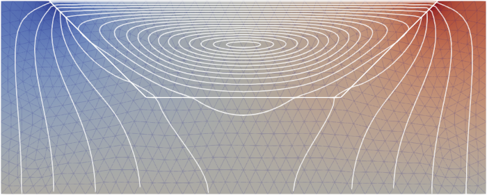
The picture shows the stream lines of the Stokes velocity \(u\) and Darcy flux \( K\nabla \varphi\) in the two subdomains and was created from the result file stokes-darcy.vtu with Paraview.

Error handling

In case an exception is thrown within main(), the function is followed by a catch block that will print the error message and exit the program with error code 1.

}
catch (Dune::Exception& e)
{
  std::cout << e.what() << std::endl;
  return 1;
}