Poisson equation with periodic BC

Table of Contents

• Introduction
• Setup and initialization
• Define problem data
• Create grid
• Setting up boundary patches
• Compute coloring for thread-parallelism
• Create finite element basis
• Create matrix, vector, and constraints data structures
• Assemble the variational problem
• Solve the algebraic problem
• Write solution to VTK
• Error handling

Full code of this example This example on gitlab

Introduction

This example solves the Poisson equation with periodic boundary conditions. In particular it demonstrates how to mark boundary subsets for the definition of periodic boundary conditions.

Setup and initialization

After including the required headers the main() function first creates a simple logger that allows to write log messages to std::cout. The logger will prefix log messages with the time passed since the program was started and since the last log message using the given format string. Then the first two command line arguments - if present - are parsed. They allow to set the number of grid refinement steps and the number of threads in parallel algorithms. Afterward MPI is initialized, passing the command line arguments.

int main (int argc, char *argv[]) try
{
 
  auto log = Dune::Fufem::makeLogger(std::cout, "[% 8.3f] [% 8.3f] ");
 
  auto parameters = Dune::ParameterTree();
  Dune::ParameterTreeParser::readOptions(argc, argv, parameters);
 
  auto refinements  = parameters.get<std::size_t>("refinements", 3);
  auto threadCount  = parameters.get<std::size_t>("threads", std::thread::hardware_concurrency());
  auto tol          = parameters.get<double>("tol", 1e-4);
  auto maxIter      = parameters.get<std::size_t>("maxIter", 1000);
  auto verbosity    = parameters.get<std::size_t>("verbosity", 2);
 
  log("Command line processed");
 
  Dune::MPIHelper::instance(argc, argv);
 
  log("MPI initialized");

Define problem data

The example solves the Poisson equation with Dirichlet and periodic boundary conditions on the unit square \( (0,1)^2 \). The problem data consisting of an indicator function for the Dirichlet boundary, the Dirichlet values, and the right-hand-side function are defined using lambda expressions.

  auto dirichletIndicator = [&](auto x) {
    return (x[1] <= 0.25) or (x[1] > 0.75);
  };
 
  auto dirichletValues = [](const auto& x){ return 0; };
 
  auto rightHandSide = [] (const auto& x) { return 20*(x[0]>=.5);};

Create grid

Instead of creating a uniform grid using a factory or reading a grid from a file, the example manually creates a mixed grid of type UGGrid<2> using a GridFactory. The grid implementation UGGrid<2> supports unstructured grid in two dimensions. After inserting nine uniformly placed vertices on the unit square, the method inserts two quadrilateral elements in the lower half and four triangular elements in the upper half of the domain.

  using Grid = Dune::UGGrid<2>;
 
  auto factory = Dune::GridFactory<Grid>();
  for(unsigned int k : Dune::range(9))
    factory.insertVertex({0.5*(k%3), 0.5*(k/3)});
  factory.insertElement(Dune::GeometryTypes::cube(2), {0, 1, 3, 4});
  factory.insertElement(Dune::GeometryTypes::cube(2), {1, 2, 4, 5});
  factory.insertElement(Dune::GeometryTypes::simplex(2), {3, 4, 6});
  factory.insertElement(Dune::GeometryTypes::simplex(2), {4, 7, 6});
  factory.insertElement(Dune::GeometryTypes::simplex(2), {4, 5, 7});
  factory.insertElement(Dune::GeometryTypes::simplex(2), {5, 8, 7});

Now we could directly create the grid. However, in preparation for setting up periodic boundary conditions, we explicitly insert BoundarySegments where degrees of freedom should later be connected periodically. Each BoundarySegment corresponds to the intersection of an element with the boundary and is identified by the list of boundary vertices. This amounts in two intersections for the left boundary \(\{0\}\times (0,1)\)

  factory.insertBoundarySegment({0, 3});
  factory.insertBoundarySegment({3, 6});

and two for the right boundary \(\{1\}\times (0,1)\), respectively.

  factory.insertBoundarySegment({2, 5});
  factory.insertBoundarySegment({5, 8});

Furthermore we create a vector that associates to each of the inserted segments (ordered according to their insertion) an id which later allows to identify different parts of the boundary.

  constexpr int leftID = 0;
  constexpr int rightID = 1;
  auto boundaryIDs = std::vector({leftID, leftID, rightID, rightID});

To match the left and right boundary, we also define a function that maps the right to the left.

  auto periodicRightToLeft = [](auto x) {
    x[0] -= 1.0;
    return x;
  };

Finally, the call to factory.createGrid() returns a std::unique_ptr referring to the newly creates grid. For simplicity the example also stores a reference to the grid.

  auto gridPtr = std::unique_ptr(factory.createGrid());
  auto& grid = *gridPtr;
 
  log("Grid created");

In general, the insertion order is only known to the GridFactory and a grid implementation may reorder the inserted BoundarySegments. Hence we need to store the boundaryIDs in a persistent form. This can be done using a Dune::Fufem::BoundaryData object. To create this object we pass the vector of ids (in insertion order) as well as the factory and the grid. The boundaryData object can later be used to query the id of an intersection using boundaryData(intersection).

  auto boundaryData = Dune::Fufem::BoundaryData(boundaryIDs, factory, grid);

The coarse grid is now refined globally and copy of the leaf grid view is stored.

Note

A GridView is a view to a subset of the grid's elements, vertices, ... that should be stored by value and can be copied cheaply. Grids in dune are in general hierarchical and composed by elements on several levels. The discretization usually lives on the set of most refined elements that is denote the leaf GridView in dune.

  grid.globalRefine(refinements);
 
  log(Dune::formatString("Grid refined %d times", refinements));
 
  auto gridView = grid.leafGridView();

Setting up boundary patches

Each boundary condition is given on a certain subset of the boundary Now we create a Dune::Fufem::BoundaryPatch for each of the three subsets: The Dirichlet boundary and the left and right periodic boundaries. To traverse the boundary we use the Dune::Fufem::Boundary class which encapsulates all boundary intersections as an iterable range. The left and right periodic BoundaryPatch are created from all insersections with the respective boundary id. The dirichlet boundary is created is from the indicator function defined above.

  auto dirichletPatch = Dune::Fufem::BoundaryPatch(gridView);
  auto periodicLeftPatch = Dune::Fufem::BoundaryPatch(gridView);
  auto periodicRightPatch = Dune::Fufem::BoundaryPatch(gridView);
  for (const auto& intersection : Dune::Fufem::Boundary(gridView))
  {
    if (dirichletIndicator(intersection.geometry().center()))
      dirichletPatch.insertFace(intersection);
    if (boundaryData(intersection) == leftID)
      periodicLeftPatch.insertFace(intersection);
    if (boundaryData(intersection) == rightID)
      periodicRightPatch.insertFace(intersection);
  }
 
  log("Boundary patches set up");

Compute coloring for thread-parallelism

Dune-fufem supports thread-parallel assembly based on a coloring of the grid view. To use this feature we need to compute such a coloring. The coloredElementRange() function from the dune-assembler module computes such a coloring and returns a partition of the grid view's elements according to the coloring. The ColoredRangeExecutor class then encapsulates the information for executing parallel algorithms based on this partition.

  auto coloredRange = Dune::Assembler::Experimental::coloredElementRange(gridView);
 
  log("Grid coloring computed");
 
  auto executor = Dune::Assembler::Experimental::ColoredRangeExecutor(coloredRange, threadCount);
 
  log(Dune::formatString("Using parallelism with %d threads", threadCount));

Create finite element basis

As a next step the program creates a global finite element basis on the GridView. The helper function lagrange<2>() declares that we want to use Lagrange finite elements of order two, while the makeBasis() function creates the basis of this type on the given GridView. Both functions are from the namespace Dune::Functions::BasisFactory which is included for simplicity.

  using namespace Dune::Functions::BasisFactory;
  auto basis = makeBasis(gridView, lagrange<2>());
 
  log(Dune::formatString("Basis created with dimension %d", basis.dimension()));

Create matrix, vector, and constraints data structures

Since the basis' indices are plain integers we next define types for flat vectors and matrices of reals numbers and create a solution and a right-hand-side vector and a stiffness matrix.

  using Vector = Dune::BlockVector<double>;
  using Matrix = Dune::BCRSMatrix<double>;
 
  auto sol = Vector();
  auto rhs = Vector();
  auto stiffnessMatrix = Matrix();

To handle the boundary conditions we create an object for storing affine constraints with respect to the basis and then fill the object. First we compute the constraints for the Dirichlet boundary conditions, then for the periodic boundary conditions. For the latter we pass the two boundary patches representing both sides of the periodic boundary and a function mapping the second to the first one.

  auto constraints = Dune::Fufem::makeAffineConstraints(basis);
 
  Dune::Fufem::computeBoundaryConstraints(constraints, basis, dirichletValues, dirichletPatch);
 
  log("Boundary constraints computed");
 
  Dune::Fufem::computePeriodicConstraints(constraints, basis, periodicLeftPatch, periodicRightPatch, periodicRightToLeft);
 
  log("Periodic constraints computed");

Assemble the variational problem

Inspired by the UFL language of the Fenics project project, dune-fufem allows to define local assemblers for linear and bilinear forms using simple expressions from the Dune::Fufem::Forms namespace. After including the namespace, we first obtain expressions for trial and test functions associated to the basis. The only difference between trialFunction() and testFunction() is that the resulting objects later refer to column and row indices, respectively. In order to use the right-hand-side lambda functions within a form expression we first wrap it into a GridView-functions and then declare this as coefficient function, i.e. a function not depending on test and trial functions. Now we can define the bilinear and linear form in a straight forward way. The defined bilinear form and linear form objects satisfy the interfaces for local matrix and vector assemblers to be passed to a global assembler.

  using namespace Dune::Fufem::Forms;
 
  auto u = trialFunction(basis);
  auto v = testFunction(basis);
  auto f = Coefficient(Dune::Functions::makeGridViewFunction(rightHandSide, gridView));
 
  auto a = integrate(dot(grad(u), grad(v)));
  auto l = integrate(f*v);

For global assembly we use the dune-assembler module. This module allows to use different linear algebra frameworks through a unified matrix- and vector-backend interface. To use the matrix- and vector-classes from dune-istl, we wrap them into corresponding ISTL-backends.

  auto matrixBackend = Dune::Assembler::ISTLMatrixBackend(stiffnessMatrix);
  auto rhsBackend = Dune::Assembler::ISTLVectorBackend(rhs);

Next we create a global assembler object using the same basis for the test and trial space. In order to use thread-parallel assembly, we additionally pass the parallel executor which encapsulates the grid coloring and requested thread count to the assembler.

  auto assembler = Dune::Assembler::Assembler(basis, basis, executor);
 
  log("Assembler set up");

As a first step we need to assemble the matrix pattern. To this end we obtain a patternBuilder object from the matrix backend and initialize its size according to the test and trial basis. Then we use the global assemblers assembleMatrixPattern() method to assemble the pattern. While local matrices are often fully populated, this is not necessarily the case. Hence the local assembler also defines a local pattern and thus has to be passed when assembling the pattern, too.

Since the periodic boundary conditions lead to constraints that require an extended matrix pattern, we next use constraints.extendMatrixPattern(...) to insert the required entries into the pattern.

  auto patternBuilder = matrixBackend.patternBuilder();
 
  patternBuilder.resize(basis, basis);
 
  assembler.assembleMatrixPattern(a, patternBuilder);
 
  constraints.extendMatrixPattern(patternBuilder, basis);
 
  log("Matrix pattern assembled");

Now we are ready to assemble the problem. To this end we let the patternBuilder initialize the matrix size and pattern and then call the actual assembly method for the matrix.

  patternBuilder.setupMatrix();
 
  log("Matrix set up");
 
  assembler.assembleMatrixEntries(a, matrixBackend);
 
  log("Matrix assembled");

Similarly we assemble the right hand side by first resizing the vector according to the test basis and initializing it with zero and then calling the corresponding assembly method.

  rhsBackend.resize(basis);
  rhsBackend.setZero();
 
  assembler.assembleVectorEntries(l, rhsBackend);
 
  log("RHS assembled");

Once the system is assembled, we can constrain it to the affine subspace satisfying the constraints that we defined earlier.

  constraints.constrainLinearSystem(stiffnessMatrix, rhs);
 
  log("Boundary condition incorporated into system");

Solve the algebraic problem

Before solving the linear system, we have to initialize the solution vector. While we could directly use the corresponding resize method and assignment operator, we here demonstrate how the ISTLVectorBackend from dune-assembler can be used, since this approach would also work for basis using multi-indices and corresponding nested vector containers.

Note

There is also a utility Dune::Functions::istlVectorBackend() provided by the dune-functions module. The Dune::Assemble::ISTLVectorBackend extends the latter by a few methods required for assembly. Here we could have used the version from the dune-functions module as well with a slightly different syntax.

  Dune::Assembler::ISTLVectorBackend(sol).resize(basis);
  Dune::Assembler::ISTLVectorBackend(sol).setZero();

To use the matrix in the solvers from the dune-istl module we first wrap it into a suitable operator interface. Then we create an AMG preconditioner and pass the operator and preconditioner to a CG solver. The apply() method of the latter solves the linear system up to the given tolerance and writes some solver statistics to the respective object that needs to be passed additionally.

  auto matrixOperator = Dune::MatrixAdapter<Matrix,Vector,Vector>(stiffnessMatrix);
 
  auto preconditioner = makeAMGPreconditioner<Vector>(stiffnessMatrix);
 
  log("Preconditioner created");
 
  auto solver = Dune::CGSolver<Vector>(
                  matrixOperator,
                  preconditioner,
                  tol,
                  maxIter,
                  verbosity
                );
 
  log("Solver created");
 
  auto solverStatistics = Dune::InverseOperatorResult();
 
  solver.apply(sol, rhs, solverStatistics);
 
  log("Linear system solved");

By constraining the linear system earlier, we have effectively only solved a problem in a suitable affine subspace. To also compute the correct coefficients for the remaining, constrained degrees of freedom, we use the constraints.interpolate(...) function which interpolates those degrees of freedom from the non-constrained ones.

  constraints.interpolate(sol);
 
  log("Constrained solution interpolated");

Write solution to VTK

Finally we can write the solution to a VTK file understood by the ParaView visualization program. To this end we need to create a finite element function by combining the basis with the coefficient vector. Here this is obtained using the expression u|sol which binds the linear operator u (i.e. the identity on the finite element space) to the coefficient vector sol. We create a writer object capable of writing unstructured grids and tell it to write polynomial data of order 2 and pass the function to the writer, specifying the name and data type of the resulting field in the output.

  auto vtkWriter = Dune::Vtk::UnstructuredGridWriter(Dune::Vtk::LagrangeDataCollector(basis.gridView(), 2));
  vtkWriter.addPointData(u|sol, Dune::VTK::FieldInfo("sol", Dune::VTK::FieldInfo::Type::scalar, 1));
  vtkWriter.write("poisson-periodic");
 
  log("Solution written to vtk file");

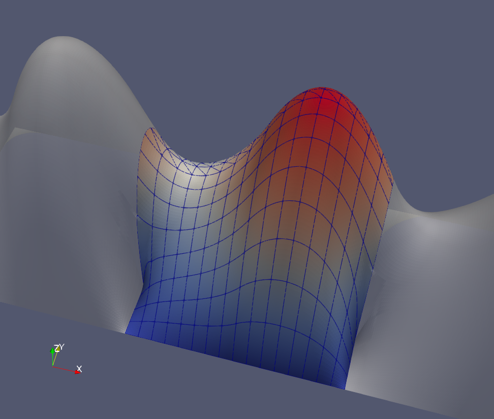
The picture shows the visualization of the written file poisson-periodic.vtu Paraview. Here we used paraview filters to additionally plot two transparent copies of the solution, shifted by to -1 and +1 to the left and right, respectively. This allows to illustrate the periodicity of the solution on the respective part of boundary.

Error handling

In case an exception is thrown within main() it is followed by a catch block that will print the error message and exit.

}
catch (Dune::Exception& e)
{
  std::cout << e.what() << std::endl;
  return 1;
}